Improving NVFP4 Accuracy with Local Hessian Weight Scales

Author:

Model Optimizer Team

Date:

September 9, 2026

Tags:

local-hessian, quantization, nvfp4, calibration, modelopt

In this blog, we share about Model Optimizer ‘Local-Hessian’, an algorithm for NVFP4 per-block scale selection to minimize the output error. We used this algorithm to create a low loss checkpoint nvidia/Qwen3.8-27B-NVFP4 which can leverage NVFP4 tensor cores for performant inference on Blackwell GPUs. Here is a comparison of accuracy results we observed for ‘Local Hessian’ algorithm compared to the default max algorithm:

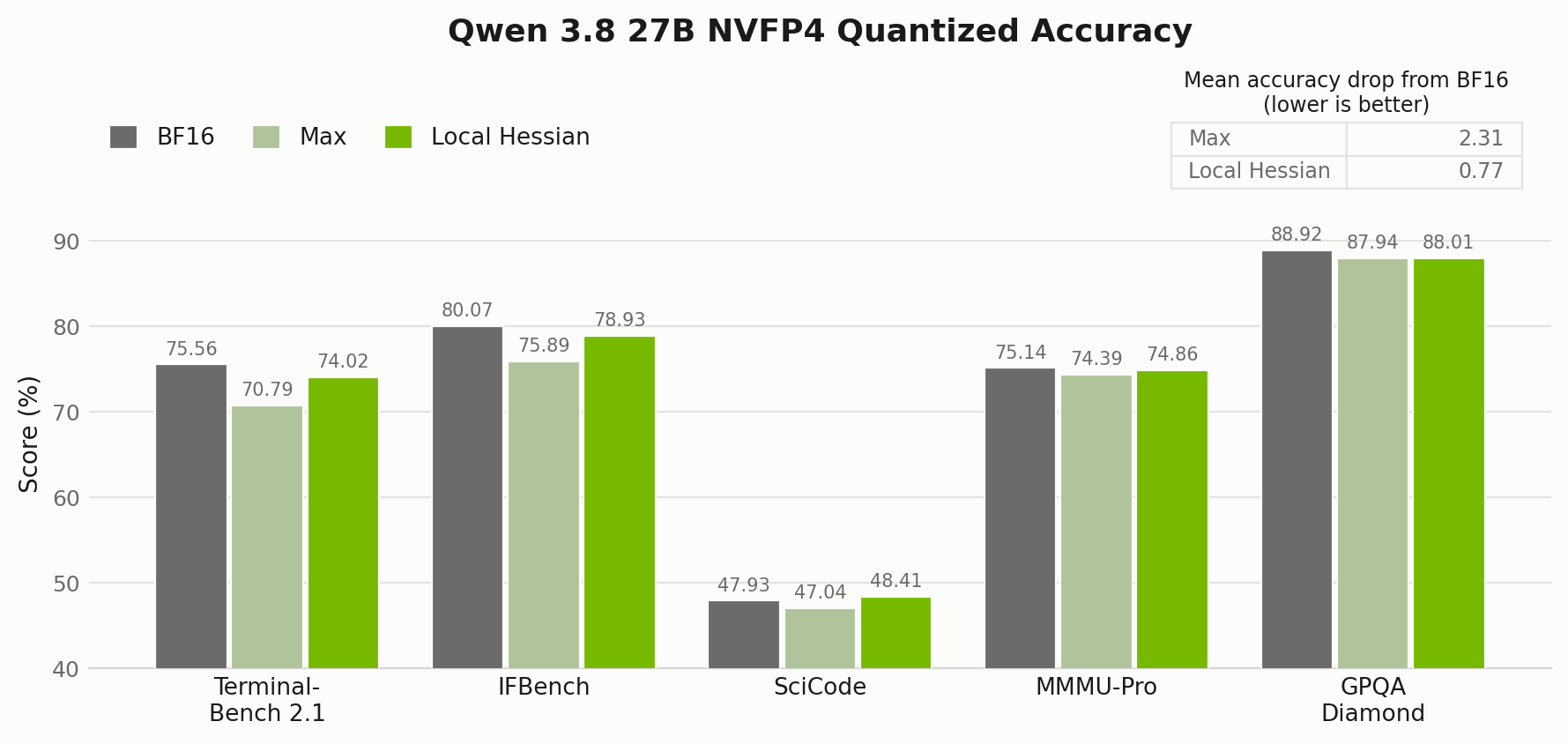
Figure 1. Qwen3.8-27B NVFP4 accuracy comparison between the default NVFP4 algorithm (max) and ‘Local-Hessian’.

Background: NVFP4 Scale Selection

NVFP4 represents each group of 16 weights with FP4 values and an FP8 block scale [1]. This block scale is used to scale the per-block values so to NVFP4 E2M1 range (-6.0, 6.0). The default way is to set the block scale based on the per-block maximum value (max scaling) [1].

As shown, originally in ‘Four-Over-Six’ paper [2], this block scale can be selected based on other critieria like per-block error. While ‘Four-Over-Six’ selects the per-block scale from 2 candidates while Model-Optimizer Mean Square Error (MSE) algorithm sets this based on exhuastive sweep over all positive and non-zero FP8 scales (126 values).

Both of these approaches for scale selection only considers weight tensor level error which we find does not correlate well with downstream accuracy evaluation results.

How Local Hessian Works

NVFP4 Local-Hessian chooses each per-block weight scale to minimize the output error of the matrix multiplication rather than the weight error. Nothing about the format changes – we just compute the per-block scales differently from max scaling.

Consider a linear layer \(Y=WX\) with weights \(W\in\mathbb{R}^{C_{\mathrm{out}}\times C_{\mathrm{in}}}\) and calibration inputs \(X\in\mathbb{R}^{C_{\mathrm{in}}\times N}\), where \(N\) is the number of calibration tokens. Quantizing divides by a scale and casts, \(\mathcal{Q}(W,s)=\operatorname{Cast}(W/s)\cdot s\), leaving an error \(\Delta(W,s)=\mathcal{Q}(W,s)-W\). Taking one output channel at a time, with its weights in the row \(w\), the output mean squared error is

(1)\[\begin{split}E(s) &= \lVert wX-w_qX\rVert_2^2 = \lVert \Delta(w,s)\,X\rVert_2^2 \\ &= \Delta(w,s)\,(XX^{\top})\,\Delta(w,s)^{\top}.\end{split}\]

The input second-moment matrix \(XX^{\top}\in\mathbb{R}^{C_{\mathrm{in}}\times C_{\mathrm{in}}}\) is the ‘Hessian’ of the output error, i.e, \(\partial^2E(s)/\partial\Delta(w,s)^2\): it weights each weight error by how much that input coordinate actually moves the output.

For NVFP4, \(s\) is not a scalar: each output channel has \(C_{\mathrm{in}}/16\) blocks, one scale each. With \(M\) candidates per block, minimizing \(E(s)\) jointly means searching \(M^{C_{\mathrm{in}}/16}\) combinations – this is not tractable. So we choose each block’s scale in isolation, against the output error that block alone contributes. For block \(b\),

(2)\[E_b(s_b) = \Delta(w_b,s_b)\,(X_bX_b^{\top})\,\Delta(w_b,s_b)^{\top},\]

where the local Hessian \(X_bX_b^{\top}\) is only \(16\times16\). For each block we sweep all 126 candidate FP8 scales, just as the MSE algorithm does. See the Model Optimizer Local-Hessian code for details.

Results

Scale Selection Accuracy

In Table 1 we compares Local-Hessian Vs other scale selection algorithms dor weights on Qwen 3.5 9B.

Local Hessian gives the overall best accuracy among the NVFP4 weight-scale selection methods, cutting the average drop from 5.10 to 3.10 points against the default max rule. We get that from nothing but a smarter way of computing the weight scale – which says something about micro-block formats like NVFP4: the scale carries a lot of information, and it pays to set it diligently.

Weight scale selection method	MMLU	HellaSwag	WinoGrande	GSM8K	Average drop (lower is better)	WikiText PPL (lower is better)
BF16 reference	78.69	78.04	73.40	87.64	0.00	9.20
Max scale	75.81	76.33	70.64	74.60	5.10	10.08
MSE scale	76.49	76.61	72.45	76.72	3.87	9.98
Four-over-six scale	75.32	76.62	70.40	76.42	4.75	10.02
Local Hessian scale	76.81	76.50	71.19	80.89	3.10	9.90

All layers except the final output layer (lm_head) use NVFP4 weight and activation quantization (W4A4).

Local-Hessian + GPTQ Accuracy

Local Hessian changes scales; GPTQ [3] changes weight rounding to minimize per-layer output error. The two are orthogonal, so they compose: Local Hessian rounds to nearest (RTN) by default, and GPTQ can replace that rounding step once the scales are set. In Table 2, we show that Local-Hessian scales improve GPTQ as well.

Two things stand out:

1. Local-Hessian scale selection alone (3.10 average drop) beats GPTQ with max scales (4.84), with no weight update at all.

2. Composing the two improves further still, from 3.10 to 2.94.

Table 2. Qwen3.5-9B, NVFP4 W4A4 GPTQ composition.

Method	MMLU	HellaSwag	WinoGrande	GSM8K	Average drop	WikiText PPL
GPTQ with max scale	75.77	76.51	70.17	75.97	4.84	10.02
GPTQ + Local Hessian scale	76.98	76.59	70.96	81.50	2.94	9.91

Just Better Scales, No Runtime Cost

Local Hessian and the other ModelOpt scale-selection algorithms for NVFP4 weight scales are free. Weight scales are computed only once, at checkpoint creation, and that same scale is reused on every deployment. Selecting scales this way improves accuracy without incurring any deployment throughput penalty.

Using Local Hessian

See the local_hessian_calibrate API for the calibration entry point.

To use it in your own configuration, set the algorithm field:

import modelopt.torch.quantization as mtq

config = {
    "quant_cfg": [...],  # quantizer configuration
    "algorithm": {
        "method": "local_hessian",
        "fp8_scale_sweep": True,
        "layerwise": {
            "enable": True,
            "get_qdq_activations_from_prev_layer": True,
        },
    },
}

model = mtq.quantize(model, config, forward_loop)

See Quantization Configuration (quant_cfg) for how to write the quant_cfg field.

To reproduce the published Qwen3.8-27B checkpoint end to end:

python examples/hf_ptq/hf_ptq.py \
    --pyt_ckpt_path Qwen/Qwen3.8-27B \
    --recipe modelopt_recipes/models/Qwen/Qwen3.8-27B/ptq/nvfp4_local_hessian-fp8_attn-kv_fp8_cast.yaml \
    --dataset nemotron-post-training-v3 \
    --calib_size 512 \
    --calib_seq 2048 \
    --batch_size 1 \
    --export_path <export_dir>

Note

We use layerwise calibration: layers are calibrated one at a time. The first layer is quantized and calibrated, its outputs are then collected with fake quantization applied, and those activations feed the next layer. Each layer therefore calibrates on the input distribution it will actually see at deployment.

Note

We set batch size 1 for calibration that depends on activation statistics – Local Hessian, GPTQ and similar – so that padding tokens do not contaminate those statistics.

Next steps

• Adapt Local Hessian for sparse MoEs. Many experts in a sparse MoE see very little calibration data. Local-Hessian workflow needs to be adapted to that low-data regime.

References

[1] (1,2)

E. Alvarez, O. Almog, E. Chung, S. Layton, D. Stosic, R. Krashinsky, and K. Aubrey. Introducing NVFP4 for Efficient and Accurate Low-Precision Inference. NVIDIA Technical Blog, 2025.

[2]

J. Cook, J. Guo, G. Xiao, Y. Lin, K. Wyss, M. Nazemi, A. Mishra, C. del Mundo, T. Blankevoort, and S. Han. Four Over Six: More Accurate NVFP4 Quantization with Adaptive Block Scaling. arXiv:2512.02010, 2025.

[3]

E. Frantar, S. Ashkboos, T. Hoefler, and D. Alistarh. GPTQ: Accurate Post-Training Quantization for Generative Pre-trained Transformers. ICLR, 2023.