B-Spline Interpolation for Particle Mesh Methods

This example demonstrates B-spline charge spreading and gathering operations used in Particle Mesh Ewald (PME) and related methods. B-splines provide smooth interpolation between particle positions and mesh grid points.

In this example you will learn:

• How B-spline basis functions work for different orders

• Spreading charges from particles to mesh grid points

• Gathering values from mesh back to particle positions

• The effect of spline order on spreading locality

• Visualizing the weight distribution in 1D and 2D

Key concepts:

• Spread: Distributes point charges to nearby mesh points using B-spline weights

• Gather: Interpolates mesh values back to arbitrary positions

• Conservation: The sum of weights equals 1 (charge is conserved)

• Center of mass: Spread weights are centered at the atom position

Important

This script is intended for visualization and understanding. For actual PME calculations, use the particle_mesh_ewald() API.

Setup and Imports

We import the B-spline functions and matplotlib for visualization.

from __future__ import annotations

import matplotlib.pyplot as plt
import numpy as np
import torch

from nvalchemiops.spline import bspline_weight, spline_gather, spline_spread

B-Spline Basis Functions

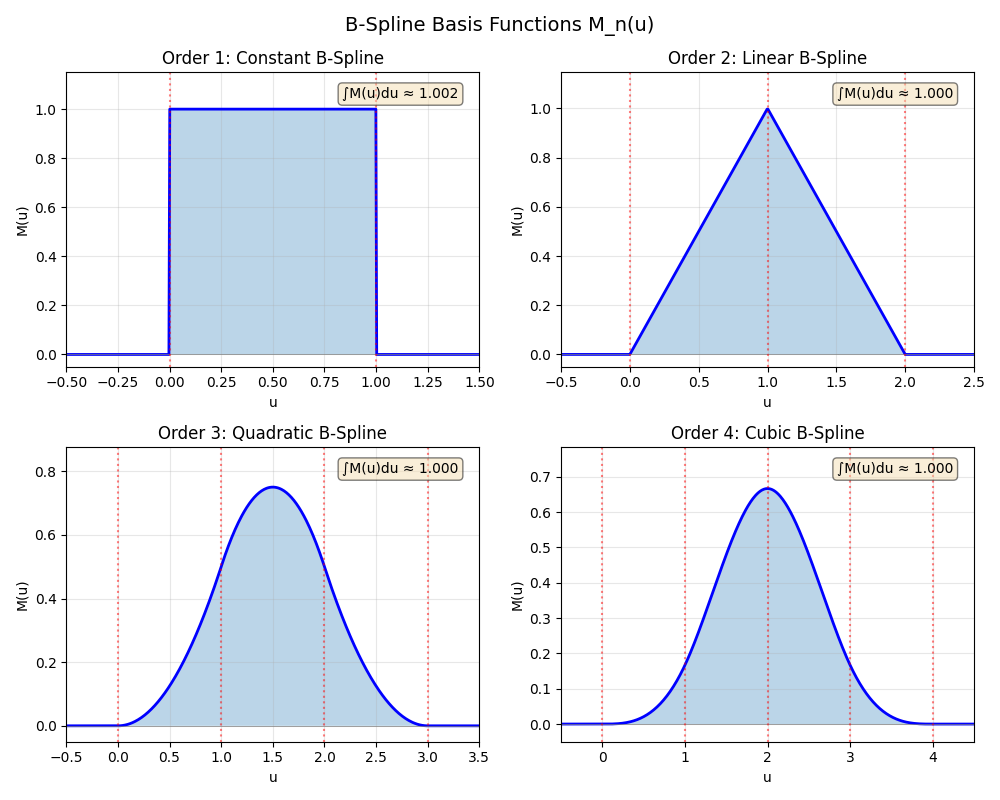
Cardinal B-splines of order n have support over [0, n) and integrate to 1. Higher orders provide smoother interpolation but spread over more grid points.

• Order 1: Constant (nearest-grid-point)

• Order 2: Linear (cloud-in-cell)

• Order 3: Quadratic

• Order 4: Cubic (most common in PME)

Plot the B-spline basis functions for orders 1-4:

fig, axes = plt.subplots(2, 2, figsize=(10, 8))
axes = axes.flatten()
orders = [1, 2, 3, 4]
order_names = ["Constant", "Linear", "Quadratic", "Cubic"]

for idx, (order, name) in enumerate(zip(orders, order_names)):
    ax = axes[idx]
    u_vals = np.linspace(-0.5, order + 0.5, 500)
    weights = np.array([bspline_weight(u, order) for u in u_vals])

    ax.plot(u_vals, weights, "b-", linewidth=2)
    ax.fill_between(u_vals, weights, alpha=0.3)
    ax.axhline(0, color="gray", linestyle="-", linewidth=0.5)

    for i in range(order + 1):
        ax.axvline(i, color="red", linestyle=":", alpha=0.5)

    ax.set_xlim(-0.5, order + 0.5)
    ax.set_ylim(-0.05, max(weights) * 1.1 + 0.05)
    ax.set_xlabel("u")
    ax.set_ylabel("M(u)")
    ax.set_title(f"Order {order}: {name} B-Spline")
    ax.grid(True, alpha=0.3)

    # Show integral (should be 1)
    integral = np.trapezoid(weights, u_vals)
    ax.text(
        0.95,
        0.95,
        f"∫M(u)du ≈ {integral:.3f}",
        transform=ax.transAxes,
        ha="right",
        va="top",
        bbox=dict(boxstyle="round", facecolor="wheat", alpha=0.5),
    )

fig.suptitle("B-Spline Basis Functions M_n(u)", fontsize=14)
plt.tight_layout()
plt.show()

1D Spreading Visualization

We visualize how a single charge spreads to nearby grid points in 1D. The weights depend on the atom’s fractional position between grid points.

cell_size = 10.0
mesh_size = 16
dx = cell_size / mesh_size
grid_pos = np.arange(mesh_size) * dx

print(f"Cell size: {cell_size} Å")
print(f"Mesh size: {mesh_size}")
print(f"Grid spacing: {dx:.4f} Å")

Cell size: 10.0 Å
Mesh size: 16
Grid spacing: 0.6250 Å

Now let’s see how weights are distributed when we place an atom at different positions. We test 4 cases: exactly on a grid point, slightly off-grid, halfway between grid points, and at the next grid point.

fig, axes = plt.subplots(2, 2, figsize=(12, 10))

# Test different atom positions
atom_positions_1d = [5.0, 5.3, 5.625, 6.0]

for ax, atom_x in zip(axes.flatten(), atom_positions_1d):
    cell = torch.diag(torch.tensor([cell_size, cell_size, 1.0], dtype=torch.float64))
    positions = torch.tensor([[atom_x, 5.0, 0.5]], dtype=torch.float64)
    charges = torch.tensor([1.0], dtype=torch.float64)

    mesh = spline_spread(positions, charges, cell, [mesh_size, mesh_size, 1], 4)
    y_idx = int(5.0 / dx)
    weights_1d = mesh[:, y_idx, 0].cpu().numpy()

    # Bar plot showing weights at each grid point
    colors = ["steelblue" if w > 1e-10 else "lightgray" for w in weights_1d]
    ax.bar(
        grid_pos,
        weights_1d,
        width=dx * 0.8,
        color=colors,
        edgecolor="black",
        linewidth=0.5,
        alpha=0.7,
    )

    # Mark atom position
    ax.axvline(
        atom_x, color="red", linewidth=2, linestyle="--", label=f"Atom at x={atom_x}"
    )
    ax.scatter([atom_x], [0], c="red", s=200, marker="*", zorder=5, clip_on=False)

    # Compute and show center of mass
    com = (grid_pos * weights_1d).sum() / weights_1d.sum()
    ax.axvline(com, color="cyan", linewidth=2, linestyle="-", label=f"COM = {com:.3f}")

    # Annotate non-zero weights
    for gp, w in zip(grid_pos, weights_1d):
        if w > 1e-10:
            ax.annotate(f"{w:.3f}", (gp, w + 0.02), ha="center", fontsize=8)

    ax.set_xlabel("Position (grid points shown as ticks)")
    ax.set_ylabel("Weight")
    ax.set_title(f"Atom at x = {atom_x:.3f}\n(mesh coord = {atom_x / dx:.2f})")
    ax.set_xlim(2, 9)
    ax.set_ylim(-0.05, max(weights_1d) * 1.3)
    ax.legend(loc="upper right", fontsize=9)
    ax.grid(True, alpha=0.3, axis="y")

fig.suptitle(
    "1D B-Spline Spreading: Weights at Grid Points\n(Order 4, Mesh 16)", fontsize=14
)
plt.tight_layout()
plt.show()

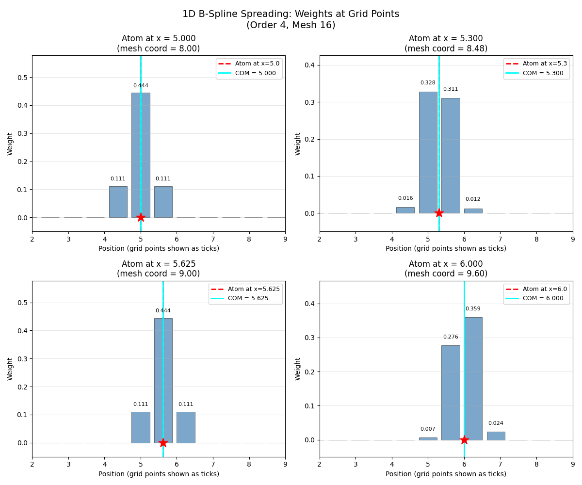
Key observation: The center of mass (cyan line) always matches the atom position (red dashed line), demonstrating that B-splines preserve the first moment of the charge distribution.

print("Weight conservation check:")
for atom_x in atom_positions_1d:
    cell = torch.diag(torch.tensor([cell_size, cell_size, 1.0], dtype=torch.float64))
    positions = torch.tensor([[atom_x, 5.0, 0.5]], dtype=torch.float64)
    charges = torch.tensor([1.0], dtype=torch.float64)
    mesh = spline_spread(positions, charges, cell, [mesh_size, mesh_size, 1], 4)
    total_weight = mesh.sum().item()
    print(f"  Atom at x={atom_x}: total weight = {total_weight:.6f}")

Weight conservation check:
  Atom at x=5.0: total weight = 1.000000
  Atom at x=5.3: total weight = 1.000000
  Atom at x=5.625: total weight = 1.000000
  Atom at x=6.0: total weight = 1.000000

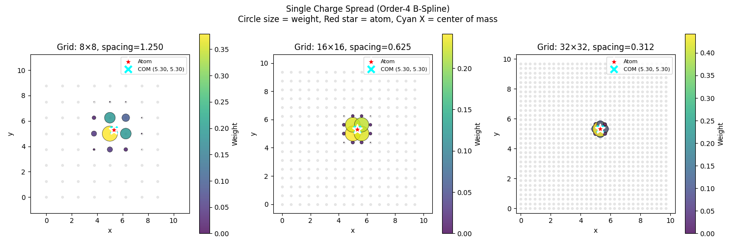
2D Spreading Visualization

We show how a single charge spreads in 2D using a scatter plot where circle size and color represent the weight at each grid point.

def visualize_spread_2d(
    positions: torch.Tensor,
    charges: torch.Tensor,
    cell: torch.Tensor,
    mesh_size: int,
    spline_order: int,
    ax: plt.Axes,
    title: str = None,
):
    """Visualize 2D spreading with scatter plot."""
    cell_size = cell[0, 0].item()
    dx = cell_size / mesh_size

    # Spread charges
    mesh = spline_spread(
        positions, charges, cell, [mesh_size, mesh_size, 1], spline_order
    )
    mesh_2d = mesh[:, :, 0].cpu().numpy()

    # Create grid point positions
    x_grid = np.arange(mesh_size) * dx
    y_grid = np.arange(mesh_size) * dx
    xx, yy = np.meshgrid(x_grid, y_grid, indexing="ij")

    x_flat = xx.flatten()
    y_flat = yy.flatten()
    weights = mesh_2d.flatten()

    # Show all grid points as small gray dots
    ax.scatter(x_flat, y_flat, c="lightgray", s=10, alpha=0.5, zorder=1)

    # Show non-zero weights as colored circles
    mask = weights > 1e-10
    if mask.any():
        max_weight = weights.max()
        sizes = (weights[mask] / max_weight) * 500

        scatter = ax.scatter(
            x_flat[mask],
            y_flat[mask],
            c=weights[mask],
            cmap="viridis",
            s=sizes,
            alpha=0.8,
            edgecolor="black",
            linewidth=0.5,
            vmin=0,
            vmax=max_weight,
            zorder=3,
        )
        plt.colorbar(scatter, ax=ax, label="Weight")

    # Show atom position
    pos_np = positions.cpu().numpy()
    ax.scatter(
        pos_np[:, 0],
        pos_np[:, 1],
        c="red",
        s=200,
        marker="*",
        edgecolor="white",
        linewidth=2,
        zorder=5,
        label="Atom",
    )

    # Compute and show center of mass
    if weights.sum() > 0:
        com_x = (mesh_2d * x_grid[:, np.newaxis]).sum() / weights.sum()
        com_y = (mesh_2d * y_grid[np.newaxis, :]).sum() / weights.sum()
        ax.scatter(
            [com_x],
            [com_y],
            c="cyan",
            s=100,
            marker="x",
            linewidth=3,
            zorder=4,
            label=f"COM ({com_x:.2f}, {com_y:.2f})",
        )

    ax.set_xlim(-dx, cell_size + dx)
    ax.set_ylim(-dx, cell_size + dx)
    ax.set_xlabel("x")
    ax.set_ylabel("y")
    ax.set_aspect("equal")
    ax.legend(loc="upper right", fontsize=8)
    if title:
        ax.set_title(title)

Visualize single charge with different mesh resolutions:

cell_size = 10.0
cell_2d = torch.diag(torch.tensor([cell_size, cell_size, 1.0], dtype=torch.float64))
positions_2d = torch.tensor([[5.3, 5.3, 0.5]], dtype=torch.float64)
charges_2d = torch.tensor([1.0], dtype=torch.float64)

fig, axes = plt.subplots(1, 3, figsize=(15, 5))
mesh_sizes = [8, 16, 32]

for ax, ms in zip(axes, mesh_sizes):
    dx = cell_size / ms
    visualize_spread_2d(
        positions_2d,
        charges_2d,
        cell_2d,
        ms,
        spline_order=4,
        ax=ax,
        title=f"Grid: {ms}×{ms}, spacing={dx:.3f}",
    )

fig.suptitle(
    "Single Charge Spread (Order-4 B-Spline)\n"
    "Circle size = weight, Red star = atom, Cyan X = center of mass",
    fontsize=12,
)
plt.tight_layout()
plt.show()

Effect of Spline Order

Higher order splines spread over more grid points but provide smoother interpolation. We compare orders 1-4 for both spreading and gathering.

def create_dipole_system(cell_size: float = 10.0):
    """Create a simple dipole system."""
    cell = torch.diag(torch.tensor([cell_size, cell_size, 1.0], dtype=torch.float64))
    positions = torch.tensor(
        [
            [cell_size * 0.35, cell_size * 0.5, 0.5],
            [cell_size * 0.65, cell_size * 0.5, 0.5],
        ],
        dtype=torch.float64,
    )
    charges = torch.tensor([1.0, -1.0], dtype=torch.float64)
    return positions, charges, cell


def visualize_gather_2d(
    mesh: torch.Tensor,
    cell: torch.Tensor,
    spline_order: int,
    n_sample: int,
    ax: plt.Axes,
    title: str = None,
):
    """Visualize 2D gathering with scatter plot."""
    cell_size = cell[0, 0].item()

    # Create sampling grid
    x = torch.linspace(
        0.05 * cell_size, 0.95 * cell_size, n_sample, dtype=torch.float64
    )
    y = torch.linspace(
        0.05 * cell_size, 0.95 * cell_size, n_sample, dtype=torch.float64
    )
    xx, yy = torch.meshgrid(x, y, indexing="ij")

    sample_pos = torch.stack(
        [
            xx.flatten(),
            yy.flatten(),
            torch.ones(n_sample * n_sample, dtype=torch.float64) * 0.5,
        ],
        dim=1,
    )

    if mesh.dim() == 2:
        mesh_3d = mesh.unsqueeze(-1)
    else:
        mesh_3d = mesh

    values = spline_gather(sample_pos, mesh_3d, cell, spline_order)
    values_2d = values.reshape(n_sample, n_sample).cpu().numpy()

    x_flat = xx.numpy().flatten()
    y_flat = yy.numpy().flatten()
    v_flat = values_2d.flatten()

    vmax = np.abs(v_flat).max()

    if vmax > 0:
        sizes = (np.abs(v_flat) / vmax) * 200 + 10
        scatter = ax.scatter(
            x_flat,
            y_flat,
            c=v_flat,
            cmap="RdBu_r",
            s=sizes,
            alpha=0.8,
            edgecolor="gray",
            linewidth=0.2,
            vmin=-vmax,
            vmax=vmax,
            zorder=3,
        )
        plt.colorbar(scatter, ax=ax, label="Interpolated value")

    ax.set_xlim(0, cell_size)
    ax.set_ylim(0, cell_size)
    ax.set_xlabel("x")
    ax.set_ylabel("y")
    ax.set_aspect("equal")
    if title:
        ax.set_title(title)

Compare spreading for different spline orders on a dipole system:

positions_dip, charges_dip, cell_dip = create_dipole_system()
mesh_size = 32

print("Dipole system:")
print(f"  Positive charge at: {positions_dip[0].numpy()}")
print(f"  Negative charge at: {positions_dip[1].numpy()}")

Dipole system:
  Positive charge at: [3.5 5.  0.5]
  Negative charge at: [6.5 5.  0.5]

Spread visualization for each order:

fig, axes = plt.subplots(2, 4, figsize=(16, 8))
orders = [1, 2, 3, 4]

for i, order in enumerate(orders):
    mesh = spline_spread(
        positions_dip, charges_dip, cell_dip, [mesh_size, mesh_size, 1], order
    )

    # Spread visualization
    ax = axes[0, i]
    mesh_2d = mesh[:, :, 0].cpu().numpy()
    dx = cell_dip[0, 0].item() / mesh_size
    x_grid = np.arange(mesh_size) * dx
    y_grid = np.arange(mesh_size) * dx
    xx, yy = np.meshgrid(x_grid, y_grid, indexing="ij")
    x_flat = xx.flatten()
    y_flat = yy.flatten()
    values = mesh_2d.flatten()

    vmax = np.abs(values).max()
    if vmax > 0:
        mask = np.abs(values) > 1e-10
        if mask.any():
            sizes = (np.abs(values[mask]) / vmax) * 300 + 20
            scatter = ax.scatter(
                x_flat[mask],
                y_flat[mask],
                c=values[mask],
                cmap="RdBu_r",
                s=sizes,
                alpha=0.8,
                edgecolor="gray",
                linewidth=0.3,
                vmin=-vmax,
                vmax=vmax,
                zorder=3,
            )
            if i == 3:  # Only add colorbar to last
                plt.colorbar(scatter, ax=ax, label="Charge density")

    # Show atom positions
    pos_np = positions_dip.cpu().numpy()
    chrg_np = charges_dip.cpu().numpy()
    for j in range(len(chrg_np)):
        color = "darkred" if chrg_np[j] > 0 else "darkblue"
        ax.scatter(
            pos_np[j, 0],
            pos_np[j, 1],
            c=color,
            s=150,
            marker="*",
            edgecolor="white",
            linewidth=1.5,
            zorder=5,
        )

    ax.set_xlim(-dx, cell_dip[0, 0].item() + dx)
    ax.set_ylim(-dx, cell_dip[0, 0].item() + dx)
    ax.set_aspect("equal")
    ax.set_title(f"Spread: Order {order}")

    # Gather visualization
    visualize_gather_2d(
        mesh,
        cell_dip,
        spline_order=order,
        n_sample=50,
        ax=axes[1, i],
        title=f"Gather: Order {order}",
    )

fig.suptitle(
    "Effect of B-Spline Order on Charge Spreading and Interpolation", fontsize=14
)
plt.tight_layout()
plt.show()

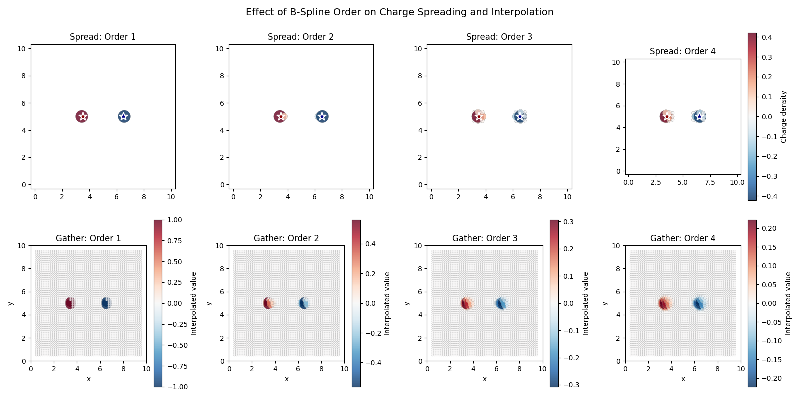
Observations:

• Order 1: Nearest-grid-point assignment, discontinuous

• Order 2: Linear interpolation, continuous but not smooth

• Order 3: Quadratic, smoother transition

• Order 4: Cubic, smooth with continuous first derivative (used in PME)

print("Number of affected grid points per dimension:")
for order in orders:
    print(f"  Order {order}: {order**3} grid points per dimension")

Number of affected grid points per dimension:
  Order 1: 1 grid points per dimension
  Order 2: 8 grid points per dimension
  Order 3: 27 grid points per dimension
  Order 4: 64 grid points per dimension

Summary

This example demonstrated:

1. B-spline basis functions of orders 1-4

2. 1D spreading showing weight distribution near an atom

3. 2D spreading visualization with scatter plots

4. Effect of mesh resolution on spreading

5. Comparison of spline orders for spreading and gathering

Key properties of B-splines in PME:

• Conservation: \(\sum_i w_i = 1\) (charge is conserved)

• Locality: Order-n spline affects n grid points per dimension

• Centering: Center of mass of weights equals atom position

• Smoothness: Higher orders give smoother potentials and forces

print("\nB-spline visualization complete!")

B-spline visualization complete!