Note
Go to the end to download the full example code
Extending Prognostic Models#
Implementing a custom prognostic model
This example will demonstrate how to extend Earth2Studio by implementing a custom prognostic model and running it in a general workflow.
In this example you will learn:
API requirements of prognostic models
Implementing a custom prognostic model
Running this model in existing workflows
Custom Prognostic#
As discussed in the Prognostic Models section of the user guide,
Earth2Studio defines a prognostic model through a simple interface
earth2studio.models.px.base.PrognosticModel. This can be used to help
guide the required APIs needed to successfully create our own custom prognostic.
In this example, let’s create a simple prognostic that simply predicts adds normal noise to the surface wind fields every time-step. While not practical, this should demonstrate the APIs one needs to implement for any prognostic.
Starting with the constructor, prognostic models should typically be torch modules.
Models need to have a to(device) method that can move the model between
different devices. If your model is PyTorch, then this will be easy.
from collections import OrderedDict
from typing import Generator, Iterator

import numpy as np
import torch

from earth2studio.models.batch import batch_func
from earth2studio.utils import handshake_coords, handshake_dim
from earth2studio.utils.type import CoordSystem


class CustomPrognostic(torch.nn.Module):
    """Custom prognostic model"""

    def __init__(self, noise_amplitude: float = 0.1):
        super().__init__()
        self.amp = noise_amplitude

    input_coords = OrderedDict(
        {
            "batch": np.empty(1),
            "lead_time": np.array([np.timedelta64(0, "h")]),
            "variable": np.array(["u10m", "v10m"]),
            "lat": np.linspace(90, -90, 721),
            "lon": np.linspace(0, 360, 1440, endpoint=False),
        }
    )

    output_coords = OrderedDict(
        {
            "batch": np.empty(1),
            "lead_time": np.array([np.timedelta64(1, "h")]),
            "variable": np.array(["u10m", "v10m"]),
            "lat": np.linspace(90, -90, 721),
            "lon": np.linspace(0, 360, 1440, endpoint=False),
        }
    )

    @batch_func()
    def __call__(
        self,
        x: torch.Tensor,
        coords: CoordSystem,
    ) -> tuple[torch.Tensor, CoordSystem]:
        """Runs prognostic model 1 step.

        Parameters
        ----------
        x : torch.Tensor
            Input tensor
        coords : CoordSystem
            Input coordinate system
        """
        for i, (key, value) in enumerate(self.input_coords.items()):
            if key != "batch":
                handshake_dim(coords, key, i)
                handshake_coords(coords, self.input_coords, key)

        out_coords = coords.copy()
        out_coords["lead_time"] = self.output_coords["lead_time"]
        out = x + self.amp * torch.rand_like(x)

        return out, out_coords

    @batch_func()
    def _default_generator(
        self, x: torch.Tensor, coords: CoordSystem
    ) -> Generator[tuple[torch.Tensor, CoordSystem], None, None]:
        """Create prognostic generator"""
        coords = coords.copy()

        for i, (key, value) in enumerate(self.input_coords.items()):
            if key != "batch":
                handshake_dim(coords, key, i)
                handshake_coords(coords, self.input_coords, key)

        # First time-step should always be the initial state
        yield x, coords

        out_coords = coords.copy()
        while True:
            out_coords["lead_time"] += self.output_coords["lead_time"]
            x = x + self.amp * torch.randn_like(x)
            yield x, out_coords

    def create_iterator(
        self, x: torch.Tensor, coords: CoordSystem
    ) -> Iterator[tuple[torch.Tensor, CoordSystem]]:
        """Creates a iterator which can be used to perform time-integration of the
        prognostic model. Will return the initial condition first (0th step).

        Parameters
        ----------
        x : torch.Tensor
            Input tensor
        coords : CoordSystem
            Input coordinate system
        """

        yield from self._default_generator(x, coords)
Input/Output Coordinates#
Defining the input/output coordinate systems is essential for any model in Earth2Studio since this is how both the package and users can learn what type of data the model expects. Have a look at Coordinate Systems for details on coordinate system. Here, we define the input output coords to be the surface winds and give the model a time-step size of 1 hour.
__call__() API#
The call function is one of the two main APIs used to interact with the prognostic model. The first thing we do is check the coordinate system of the input data is indeed what the model expects. Next, we execute the forward pass of our model (apply noise) and then update the output coordinate system.
Note
You may notice the batch_func() decorator, which is used to make batched
operations easier. For more details about this refer to the batch_function_userguide
section of the user guide.
create_iterator() API#
The call function is useful for a single time-step. However, prognostics generate time-series which is done using an iterator. This is achieved by creating a generator under the hood of the prognostic.
A generator in Python is essentially a function that returns an iterator using the
yield keyword. In the case of prognostics, it yields a single time-step
prediction of the model. Note that this allows the model to control its own internal
state inside the iterator independent of the workflow.
Since this model is auto regressive, it can theoretically index in time forever. Thus, we make the generator an infinite loop. Keep in mind that generators execute on demand, so this infinite loop won’t cause the program to get stuck.
Set Up#
With the custom prognostic defined, it’s now easily usable in a standard workflow. In
this example, we will use the build in workflow earth2studio.run.deterministic().
Let’s instantiate the components needed.
Prognostic Model: Use our custom prognostic defined above.
Datasource: Pull data from the GFS data api
earth2studio.data.GFS.IO Backend: Save the outputs into a Zarr store
earth2studio.io.ZarrBackend.
from collections import OrderedDict

import numpy as np
from dotenv import load_dotenv

load_dotenv()  # TODO: make common example prep function

from earth2studio.data import GFS
from earth2studio.io import ZarrBackend

# Create the prognostic
model = CustomPrognostic(noise_amplitude=10.0)

# Create the data source
data = GFS()

# Create the IO handler, store in memory
io = ZarrBackend()
Execute the Workflow#
Because the prognostic meets the needs of the interface, the workflow will execute just like any other model.
import earth2studio.run as run

nsteps = 24
io = run.deterministic(["2024-01-01"], nsteps, model, data, io)

print(io.root.tree())
2024-04-19 00:36:42.172 | INFO     | earth2studio.run:deterministic:68 - Running simple workflow!
2024-04-19 00:36:42.173 | INFO     | earth2studio.run:deterministic:71 - Inference device: cuda
2024-04-19 00:36:42.173 | DEBUG    | earth2studio.data.gfs:fetch_gfs_dataarray:151 - Fetching GFS index file: 2024-01-01 00:00:00

Fetching GFS for 2024-01-01 00:00:00:   0%|          | 0/2 [00:00<?, ?it/s]

2024-04-19 00:36:42.598 | DEBUG    | earth2studio.data.gfs:fetch_gfs_dataarray:197 - Fetching GFS grib file for variable: u10m at 2024-01-01 00:00:00

Fetching GFS for 2024-01-01 00:00:00:   0%|          | 0/2 [00:00<?, ?it/s]

2024-04-19 00:36:42.619 | DEBUG    | earth2studio.data.gfs:fetch_gfs_dataarray:197 - Fetching GFS grib file for variable: v10m at 2024-01-01 00:00:00

Fetching GFS for 2024-01-01 00:00:00:   0%|          | 0/2 [00:00<?, ?it/s]
Fetching GFS for 2024-01-01 00:00:00: 100%|██████████| 2/2 [00:00<00:00, 50.43it/s]
2024-04-19 00:36:42.653 | SUCCESS  | earth2studio.run:deterministic:82 - Fetched data from GFS
2024-04-19 00:36:42.674 | INFO     | earth2studio.run:deterministic:104 - Inference starting!

Running inference:   0%|          | 0/25 [00:00<?, ?it/s]
Running inference:   8%|▊         | 2/25 [00:00<00:02, 10.74it/s]
Running inference:  16%|█▌        | 4/25 [00:00<00:02,  9.19it/s]
Running inference:  20%|██        | 5/25 [00:00<00:02,  8.84it/s]
Running inference:  24%|██▍       | 6/25 [00:00<00:02,  8.32it/s]
Running inference:  28%|██▊       | 7/25 [00:00<00:02,  8.14it/s]
Running inference:  32%|███▏      | 8/25 [00:00<00:02,  7.87it/s]
Running inference:  36%|███▌      | 9/25 [00:01<00:02,  7.79it/s]
Running inference:  40%|████      | 10/25 [00:01<00:02,  7.30it/s]
Running inference:  44%|████▍     | 11/25 [00:01<00:02,  6.95it/s]
Running inference:  48%|████▊     | 12/25 [00:01<00:01,  6.77it/s]
Running inference:  52%|█████▏    | 13/25 [00:01<00:01,  6.59it/s]
Running inference:  56%|█████▌    | 14/25 [00:01<00:01,  6.38it/s]
Running inference:  60%|██████    | 15/25 [00:02<00:01,  6.26it/s]
Running inference:  64%|██████▍   | 16/25 [00:02<00:01,  6.16it/s]
Running inference:  68%|██████▊   | 17/25 [00:02<00:01,  6.07it/s]
Running inference:  72%|███████▏  | 18/25 [00:02<00:01,  5.86it/s]
Running inference:  76%|███████▌  | 19/25 [00:02<00:01,  5.69it/s]
Running inference:  80%|████████  | 20/25 [00:02<00:00,  5.51it/s]
Running inference:  84%|████████▍ | 21/25 [00:03<00:00,  5.37it/s]
Running inference:  88%|████████▊ | 22/25 [00:03<00:00,  5.32it/s]
Running inference:  92%|█████████▏| 23/25 [00:03<00:00,  5.18it/s]
Running inference:  96%|█████████▌| 24/25 [00:03<00:00,  5.05it/s]
Running inference: 100%|██████████| 25/25 [00:03<00:00,  4.94it/s]
Running inference: 100%|██████████| 25/25 [00:03<00:00,  6.29it/s]
2024-04-19 00:36:46.651 | SUCCESS  | earth2studio.run:deterministic:112 - Inference complete
/
 ├── lat (721,) float64
 ├── lead_time (25,) timedelta64[h]
 ├── lon (1440,) float64
 ├── time (1,) datetime64[ns]
 ├── u10m (1, 25, 721, 1440) float32
 └── v10m (1, 25, 721, 1440) float32
Post Processing#
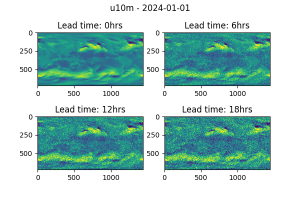
To confirm that our prognostic model is working as expected, we should see the fields become progressively more noisy as time progresses.
import os

os.makedirs("outputs", exist_ok=True)
import matplotlib.pyplot as plt

forecast = "2024-01-01"
variable = "u10m"

plt.close("all")

# Create a figure and axes with the specified projection
fig, ax = plt.subplots(2, 2, figsize=(6, 4))

# Plot u10m every 6 hours
ax[0, 0].imshow(io[variable][0, 0], vmin=-20, vmax=20)
ax[0, 1].imshow(io[variable][0, 6], vmin=-20, vmax=20)
ax[1, 0].imshow(io[variable][0, 12], vmin=-20, vmax=20)
ax[1, 1].imshow(io[variable][0, 18], vmin=-20, vmax=20)


# Set title
plt.suptitle(f"{variable} - {forecast}")
times = io["lead_time"].astype("timedelta64[h]").astype(int)
ax[0, 0].set_title(f"Lead time: {times[0]}hrs")
ax[0, 1].set_title(f"Lead time: {times[6]}hrs")
ax[1, 0].set_title(f"Lead time: {times[12]}hrs")
ax[1, 1].set_title(f"Lead time: {times[18]}hrs")

plt.savefig("outputs/custom_prognostic_prediction.jpg", bbox_inches="tight")
Total running time of the script: (0 minutes 5.332 seconds)