Variable-Cell L-BFGS Optimization (FCC Argon)

Joint relaxation of atomic coordinates and the simulation cell with the L-BFGS optimizer, using the PyTorch binding nvalchemiops.torch.lbfgs.lbfgs_step_coord_cell().

Compared with the FIRE2 variable-cell example (11_fire2_variable_cell.py), the L-BFGS path is a single call and takes the stress directly:

• You pass stress; the optimizer converts it to a cell driving force internally, so there is no separate stress_to_cell_force step

• The same stress is used for the stress convergence criterion, which is compared against a real stress rather than against a packed cell force

• There is no timestep or cell mass to tune

How the coupling works

Positions and cell are mapped into one packed coordinate vector, so the quasi-Newton recursion couples them with no special handling. The coordinates follow ASE’s UnitCellFilter convention: with a reference cell H0 fixed at the start and lattice vectors held as columns, the deformation gradient is Phi = H H0^-1, atoms are stored as u = Phi^-1 r and the cell as kappa * Phi.

Two consequences are worth knowing:

• The cell must be aligned with align_cell before the first step, exactly as fire2_step_coord_cell requires, and the six packed cell components are the same six FIRE2 packs.

• The reference cell is captured once, by lbfgs_prepare_cell_state. Rebuilding the chart mid-run invalidates every stored curvature pair, because they compare cell coordinates across steps. This is the one rule FIRE2 does not share: it keeps no history.

• The optimizer buffers must be sized for num_atoms + 2 * num_systems degrees of freedom, because the cell contributes two packed entries per system.

The preparation functions allocate and initialize both states, but the packed topology stays yours: this example builds it with the generic batch utilities, which is what makes ragged batches (systems with different atom counts) expressible.

Apply your thresholds to the Cartesian forces and the stress, never to the packed norms, so they keep their physical meaning however far the cell deforms.

The full set of cell rules – alignment, the six-component convention, the fixed reference, topology, and ragged and empty systems – is stated once in the nvalchemiops.dynamics.optimizers.lbfgs module documentation. This example follows it rather than restating it.

from __future__ import annotations

import matplotlib.pyplot as plt
import numpy as np
import torch
import warp as wp
from _dynamics_utils import (
    EPSILON_AR,
    SIGMA_AR,
    MDSystem,
    create_fcc_lattice,
    pressure_ev_per_a3_to_gpa,
    pressure_gpa_to_ev_per_a3,
    virial_to_stress,
)

from nvalchemiops.dynamics.utils import align_cell, wrap_positions_to_cell
from nvalchemiops.torch.lbfgs import (
    lbfgs_prepare_cell_state,
    lbfgs_prepare_state,
    lbfgs_step_coord_cell,
)

CUTOFF = 2.5 * SIGMA_AR  # ~8.5 Å

wp.init()
device = "cuda:0" if wp.is_cuda_available() else "cpu"
torch_device = torch.device(device)
print(f"Using device: {device}")

Warp UserWarning: Kernel cache artifacts from a previous Warp version were found in '/tmp/warp-cache'. These will be ignored. You can safely delete them.
Using device: cuda:0

Create Initial System

An FCC argon lattice, deliberately expanded from its equilibrium spacing so there is something for the cell to relax.

n_cells = 3  # 3x3x3 = 108 atoms
a_initial = 5.5  # Å (equilibrium is near 5.26 Å)

positions_np, cell_np = create_fcc_lattice(n_cells, a_initial)
num_atoms = len(positions_np)
num_systems = 1

target_pressure_gpa = 0.01
target_pressure = pressure_gpa_to_ev_per_a3(target_pressure_gpa)

print(f"System: {num_atoms} atoms in {n_cells}³ FCC lattice")
print(f"Initial lattice constant: {a_initial:.3f} Å")
print(f"Target external pressure: {target_pressure_gpa:.3f} GPa")

positions = wp.array(positions_np, dtype=wp.vec3d, device=device)
cell = wp.array(cell_np.reshape(1, 3, 3), dtype=wp.mat33d, device=device)

md_system = MDSystem(
    positions=positions_np,
    cell=cell_np,
    epsilon=EPSILON_AR,
    sigma=SIGMA_AR,
    cutoff=CUTOFF,
    skin=0.5,
    switch_width=1.0,  # smooth cutoff, so the energy is differentiable
    device=device,
)

System: 108 atoms in 3³ FCC lattice
Initial lattice constant: 5.500 Å
Target external pressure: 0.010 GPa
Initialized MD system with 108 atoms
  Cell: 16.50 x 16.50 x 16.50 Å
  Cutoff: 8.50 Å (+ 0.50 Å skin)
  LJ: ε = 0.0104 eV, σ = 3.40 Å
  Device: cuda:0, dtype: <class 'numpy.float64'>
  Units: x [Å], t [fs], E [eV], m [eV·fs²/Ų] (from amu), v [Å/fs]

Align the Cell, Once

The optimizer keeps the cell in its aligned form, stopping it drifting into a rotation. Align before capturing the reference cell: re-aligning mid-run redefines the chart and invalidates the history.

transform = wp.empty(1, dtype=wp.mat33d, device=device)
positions, cell = align_cell(positions, cell, transform=transform, device=device)
wp.copy(md_system.wp_positions, positions)
md_system.update_cell(cell)

# Wrap once, before the first step. Wrapping *during* the run teleports atoms
# across the boundary, and that discontinuity corrupts the curvature pairs.
# FIRE2 tolerates per-step wrapping because it carries no history.
wrap_positions_to_cell(
    positions=md_system.wp_positions,
    cells=md_system.wp_cell,
    cells_inv=md_system.wp_cell_inv,
    device=device,
)
wp.synchronize()
print(f"\nAligned cell:\n{cell.numpy()[0]}")

Aligned cell:
[[16.5  0.   0. ]
 [ 0.  16.5  0. ]
 [ 0.   0.  16.5]]

Prepare the Two States

Two objects, both yours: an LBFGSState as on the coordinate-only path, and an LBFGSCellState carrying the chart and its scratch. The preparation functions allocate, initialize and validate both; every field stays reachable by name.

# Work on the system's own arrays, so in-place writes are visible to the force
# engine. Only the cell needs handing back: its inverse and the neighbor list
# depend on it.
positions_t = wp.to_torch(md_system.wp_positions)
cell_t = wp.to_torch(cell).reshape(num_systems, 3, 3)
batch_idx = torch.zeros(num_atoms, dtype=torch.int32, device=torch_device)

dtype, i32 = torch.float64, torch.int32
history_size = 6
# The cell contributes two packed entries per system, so the optimizer state is
# sized for num_atoms + 2 * num_systems degrees of freedom, not num_atoms.
num_dofs = num_atoms + 2 * num_systems

# Every per-system scalar follows the coordinate dtype, so this is an fp64
# state end to end; passing float32 would give an fp32 one.
state = lbfgs_prepare_state(
    num_dofs,
    num_systems,
    dtype=dtype,
    history_size=history_size,
    device=torch_device,
)

Prepare the Variable-Cell Chart

One call. Hand it the ordinary atom_ptr you already have and the aligned cells, and it derives the packed topology, captures the reference cell that defines the chart, and computes kappa – the state comes back ready to step, with nothing left to repair.

Deriving the topology costs no generality: atom_ptr already carries each system’s atom count, so ragged batches work exactly as before. kappa scales the cell coordinate against the atomic ones; raise cell_force_scale to make the cell move less per step.

atom_ptr = torch.arange(num_systems + 1, dtype=i32, device=torch_device) * num_atoms

cell_state = lbfgs_prepare_cell_state(
    atom_ptr,
    cell_t,
    cell_force_scale=1.0 / num_atoms,
    dtype=dtype,
    device=torch_device,
)


print(f"\nOptimizer degrees of freedom: {num_atoms} atoms + {2 * num_systems} cell")

Optimizer degrees of freedom: 108 atoms + 2 cell

Optimization Loop

One force/stress evaluation per call. The optimizer owns neither tolerance and reports no terminal status, so the loop below applies both thresholds itself. Both are physical, and both are applied to the Cartesian forces and the stress rather than to the packed norms: force_tol is eV/Å on the largest per-atom force, stress_tol is a stress.

max_evals = 200
force_tol = 1e-4  # eV/Å
stress_tol = pressure_gpa_to_ev_per_a3(0.03)  # 0.03 GPa
maxstep = 0.2  # Å

energy_hist: list[float] = []
max_force_hist: list[float] = []
volume_hist: list[float] = []
pressure_hist: list[float] = []

print("\n" + "=" * 95)
print("VARIABLE-CELL L-BFGS OPTIMIZATION (FCC argon)")
print("=" * 95)
print(f"{'eval':>6} {'PE (eV)':>14} {'max|F|':>11} {'|stress| GPa':>13} {'a (Å)':>9}")

n_evals = 0
converged = False

for step in range(max_evals):
    energies, forces, virial = md_system.compute_forces_virial()
    stress = virial_to_stress(virial, md_system.wp_cell, target_pressure, device)
    n_evals += 1

    # Both criteria are the caller's, and both are physical: they are applied
    # to the *Cartesian* forces and the stress, never to packed norms, so they
    # keep their meaning however far the cell deforms. Tested before stepping.
    forces_t = wp.to_torch(forces)
    stress_t = wp.to_torch(stress).reshape(num_systems, 3, 3)
    fmax_now = float(forces_t.norm(dim=1).max())
    smax_now = float(np.linalg.svd(stress.numpy()[0], compute_uv=False).max())
    converged = fmax_now < force_tol and smax_now < stress_tol

    if step < 20 or step % 25 == 0 or converged:
        volume = float(np.linalg.det(cell_t.detach().cpu().numpy()[0]))
        stress_np = stress.numpy()[0]
        stress_gpa = pressure_ev_per_a3_to_gpa(0.5 * (stress_np + stress_np.T))
        stress_residual = float(np.linalg.svd(stress_gpa, compute_uv=False).max())
        pe = float(energies.numpy().sum())

        energy_hist.append(pe)
        max_force_hist.append(fmax_now)
        volume_hist.append(volume)
        pressure_hist.append(stress_residual)
        print(
            f"{step:>6d} {pe:>14.6f} {fmax_now:>11.3e} {stress_residual:>13.3e} "
            f"{(volume / (n_cells**3)) ** (1 / 3):>9.4f}"
        )

    if converged:
        break

    lbfgs_step_coord_cell(
        positions_t,
        cell_t,
        forces_t,
        stress_t,
        state,
        cell_state,
        batch_idx,
        maxstep=maxstep,
    )

    # Positions were written in place; the cell needs handing back so its
    # inverse is recomputed and the neighbor list is rebuilt.
    md_system.update_cell(cell)

# The loop tests before stepping, so on the converged path the last values
# logged already describe the geometry and cell we are keeping. If the budget
# ran out instead, the loop's final act was a *step*, and those values describe
# the point before it -- while `cell_t` below is the post-step cell. Pairing
# them would report a lattice constant and a force from two different
# geometries. Re-evaluate once so everything below agrees. This is a reporting
# evaluation, so it is deliberately not counted in `n_evals`.
if not converged:
    energies, forces, virial = md_system.compute_forces_virial()
    stress = virial_to_stress(virial, md_system.wp_cell, target_pressure, device)
    fmax_now = float(wp.to_torch(forces).norm(dim=1).max())
    stress_np = stress.numpy()[0]
    stress_gpa = pressure_ev_per_a3_to_gpa(0.5 * (stress_np + stress_np.T))
    energy_hist.append(float(energies.numpy().sum()))
    max_force_hist.append(fmax_now)
    volume_hist.append(float(np.linalg.det(cell_t.detach().cpu().numpy()[0])))
    pressure_hist.append(float(np.linalg.svd(stress_gpa, compute_uv=False).max()))

===============================================================================================
VARIABLE-CELL L-BFGS OPTIMIZATION (FCC argon)
===============================================================================================
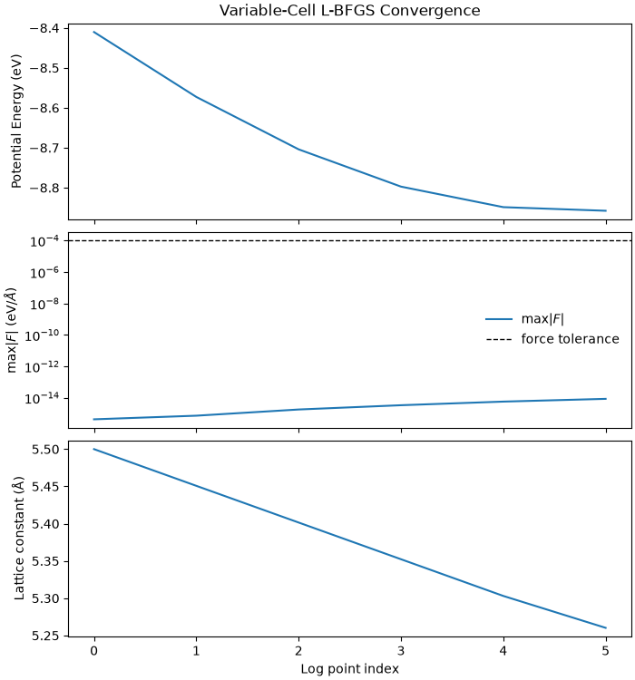
  eval        PE (eV)      max|F|  |stress| GPa     a (Å)
     0      -8.410375   4.297e-16     2.434e-01    5.5000
     1      -8.572777   7.297e-16     2.100e-01    5.4508
     2      -8.703961   1.810e-15     1.660e-01    5.4015
     3      -8.797196   3.380e-15     1.117e-01    5.3523
     4      -8.848598   5.744e-15     5.293e-02    5.3031
     5      -8.857636   8.593e-15     4.860e-03    5.2602

Result

outcome = "CONVERGED" if converged else "ran out of evaluations"

final_volume = float(np.linalg.det(cell_t.detach().cpu().numpy()[0]))
final_a = (final_volume / (n_cells**3)) ** (1 / 3)
print(f"\nFinished after {n_evals} evaluations: {outcome}")
print(f"  lattice constant: {a_initial:.4f} Å -> {final_a:.4f} Å")
# All four of these describe the same, final geometry on both paths.
print(f"  final max|F|    : {max_force_hist[-1]:.3e} eV/Å")
print(f"  final volume    : {final_volume:.2f} ų")
print(f"  final |stress|  : {pressure_hist[-1]:.4f} GPa")
print("  (textbook FCC argon equilibrium is near 5.26 Å)")

Finished after 6 evaluations: CONVERGED
  lattice constant: 5.5000 Å -> 5.2602 Å
  final max|F|    : 8.593e-15 eV/Å
  final volume    : 3929.91 ų
  final |stress|  : 0.0049 GPa
  (textbook FCC argon equilibrium is near 5.26 Å)

Plot convergence

Energy is plotted for interest, not as a convergence signal: with no Armijo test forcing it down it may rise on a step. The force is what converges.

points = np.arange(len(energy_hist))
fig, ax = plt.subplots(3, 1, figsize=(7.0, 7.5), sharex=True, constrained_layout=True)

ax[0].plot(points, energy_hist, lw=1.5)
ax[0].set_ylabel("Potential Energy (eV)")
ax[0].set_title("Variable-Cell L-BFGS Convergence")

ax[1].semilogy(points, max_force_hist, lw=1.5, label=r"max$|F|$")
ax[1].axhline(force_tol, color="k", ls="--", lw=1.0, label="force tolerance")
ax[1].set_ylabel(r"max$|F|$ (eV/$\AA$)")
ax[1].legend(frameon=False, loc="best")

ax[2].plot(points, [(v / n_cells**3) ** (1 / 3) for v in volume_hist], lw=1.5)
ax[2].set_xlabel("Log point index")
ax[2].set_ylabel("Lattice constant (Å)")

plt.show()