L-BFGS Geometry Optimization (LJ Cluster)

This example demonstrates geometry optimization with the L-BFGS optimizer using:

• The package LJ implementation (neighbor-list accelerated)

• The package L-BFGS kernels (nvalchemiops.dynamics.optimizers.lbfgs_step())

• The shared example utilities in examples.dynamics._dynamics_utils

L-BFGS is a quasi-Newton method: it builds an implicit approximation to the inverse Hessian from the last few position and force differences, then steps along that direction as far as a maxstep trust region allows. There is no line search, and no energy is read at all. Compared with FIRE2 (09_fire2_optimization.py) it:

• Reaches a given force tolerance in far fewer force evaluations, which is the cost that dominates relaxation with a machine-learned potential

• Needs no timestep to tune; the maxstep trust region bounds the step

• Costs more memory: 2 * history_size vectors of stored history

Like FIRE2, it owns no tolerance and reports no terminal status. Each call updates the curvature history, restarts the direction if it stops descending, and takes one bounded step; testing convergence and ending the loop are yours.

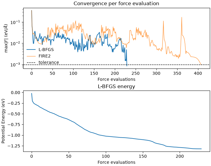
To make that first point concrete, this example relaxes the same cluster with both optimizers and compares how many force evaluations each needed.

from __future__ import annotations

import matplotlib.pyplot as plt
import numpy as np
import torch
import warp as wp
from _dynamics_utils import MDSystem, create_random_cluster

from nvalchemiops.dynamics.optimizers import (
    fire2_step,
    lbfgs_prepare_state,
    lbfgs_step,
)

wp.init()

device = "cuda:0" if wp.is_cuda_available() else "cpu"
print(f"Using device: {device}")

Warp UserWarning: Kernel cache artifacts from a previous Warp version were found in '/tmp/warp-cache'. These will be ignored. You can safely delete them.
Using device: cuda:0

Create a Lennard-Jones Cluster

num_atoms = 32
epsilon = 0.0104  # eV (argon-like)
sigma = 3.40  # Å
cutoff = 2.5 * sigma
skin = 0.5
box_L = 80.0  # Å (large to avoid self-interaction across PBC)

cell = np.eye(3, dtype=np.float64) * box_L
initial_positions = create_random_cluster(
    num_atoms=num_atoms,
    radius=12.0,
    min_dist=0.9 * sigma,
    center=np.array([0.5 * box_L, 0.5 * box_L, 0.5 * box_L]),
    seed=42,
)


def make_system() -> MDSystem:
    """A fresh system at the same starting geometry, for a fair comparison."""
    return MDSystem(
        positions=initial_positions.copy(),
        cell=cell,
        masses=np.full(num_atoms, 39.948, dtype=np.float64),  # amu (argon)
        epsilon=epsilon,
        sigma=sigma,
        cutoff=cutoff,
        skin=skin,
        switch_width=0.0,
        device=device,
        dtype=np.float64,
    )


system = make_system()
wp_dtype = system.wp_dtype
wp_vec_dtype = system.wp_vec_dtype

Initialized MD system with 32 atoms
  Cell: 80.00 x 80.00 x 80.00 Å
  Cutoff: 8.50 Å (+ 0.50 Å skin)
  LJ: ε = 0.0104 eV, σ = 3.40 Å
  Device: cuda:0, dtype: <class 'numpy.float64'>
  Units: x [Å], t [fs], E [eV], m [eV·fs²/Ų] (from amu), v [Å/fs]

Prepare the L-BFGS State

lbfgs_prepare_state() allocates and initializes every array the optimizer needs and hands them back as an LBFGSState. Calling it again is how you restart. It is a plain dataclass, so every field stays reachable – state.alpha_step, state.history_count – and you can build one from arrays you already own instead, then call state.validate().

history_size is the memory knob; 3 to 7 is usual. Coordinates may be single or double precision, but every per-system scalar is float64 regardless: ys / yy scales the initial inverse Hessian, and near convergence it is a ratio of differences of nearly equal vectors.

history_size = 6
state = lbfgs_prepare_state(
    num_atoms, 1, dtype=wp_vec_dtype, history_size=history_size, device=device
)

# Batching metadata: all zeros for a single system.
batch_idx = wp.zeros(num_atoms, dtype=wp.int32, device=device)

L-BFGS Optimization Loop

You own the loop, as with FIRE2, and each call consumes exactly one force evaluation. You also own the stopping rule: the optimizer has no tolerance and no terminal status, so the loop below tests the forces itself. No energy is passed in either – the step length comes from the maxstep trust region, so a model whose forces are not the gradient of its energy relaxes just as well.

max_evals = 500
force_tolerance = 1e-3  # eV/Å, on the largest per-atom force
maxstep = 0.2  # Å, the furthest any atom may move in one step

energy_hist: list[float] = []
maxf_hist: list[float] = []
alpha_hist_log: list[float] = []

print("\n" + "=" * 95)
print("L-BFGS GEOMETRY OPTIMIZATION (LJ cluster)")
print("=" * 95)
print(f"  atoms: {num_atoms}, cutoff={cutoff:.2f} Å, box={box_L:.1f} Å")
print(f"  history_size={history_size}, force_tol={force_tolerance:.2e} eV/Å")
print(f"  maxstep={maxstep} Å")

log_interval = 10
lbfgs_evals = 0

lbfgs_converged = False

for step in range(max_evals):
    # One force evaluation per step. This is the expensive part with a
    # real potential, and the reason L-BFGS is worth its extra bookkeeping.
    energies = system.compute_forces()
    lbfgs_evals += 1

    # Convergence is yours, exactly as it is for FIRE2: the optimizer owns no
    # tolerance and never decides you are finished. Test *before* stepping --
    # these forces describe the geometry you have, and after a step they would
    # describe the previous one.
    forces_np = system.wp_forces.numpy()
    current_fmax = float(np.linalg.norm(forces_np, axis=1).max())

    pe = float(energies.numpy().sum())
    energy_hist.append(pe)
    maxf_hist.append(current_fmax)
    alpha_hist_log.append(float(state.alpha_step.numpy()[0]))

    if step % log_interval == 0:
        print(
            f"eval={step:4d}  PE={pe:12.6f} eV  max|F|={current_fmax:10.3e} eV/Å  "
            f"alpha={alpha_hist_log[-1]:9.3e}  "
            f"iter={int(state.iteration.numpy()[0]):3d}  "
            f"hist={int(state.history_count.numpy()[0]):2d}"
        )

    if current_fmax < force_tolerance:
        lbfgs_converged = True
        break

    lbfgs_step(
        positions=system.wp_positions,
        forces=system.wp_forces,
        state=state,
        batch_idx=batch_idx,
        maxstep=maxstep,
    )

# The loop tests before stepping, so on the converged path the last values
# logged already describe the geometry we are keeping. If the budget ran out
# instead, the loop's final act was a *step*, and the last logged values
# describe the point before it. Re-evaluate once so everything reported below
# refers to the positions actually returned. This evaluation is for reporting,
# not optimization, so it is deliberately not counted in `lbfgs_evals` -- that
# number is the head-to-head metric against FIRE2.
if not lbfgs_converged:
    energies = system.compute_forces()
    energy_hist.append(float(energies.numpy().sum()))
    maxf_hist.append(float(np.linalg.norm(system.wp_forces.numpy(), axis=1).max()))
    alpha_hist_log.append(float(state.alpha_step.numpy()[0]))

===============================================================================================
L-BFGS GEOMETRY OPTIMIZATION (LJ cluster)
===============================================================================================
  atoms: 32, cutoff=8.50 Å, box=80.0 Å
  history_size=6, force_tol=1.00e-03 eV/Å
  maxstep=0.2 Å
eval=   0  PE=   -0.022508 eV  max|F|= 3.541e-01 eV/Å  alpha=1.000e+00  iter= -1  hist= 0
eval=  10  PE=   -0.328720 eV  max|F|= 1.647e-02 eV/Å  alpha=1.000e+00  iter=  9  hist= 6
eval=  20  PE=   -0.420102 eV  max|F|= 2.895e-02 eV/Å  alpha=7.697e-01  iter= 19  hist= 6
eval=  30  PE=   -0.496027 eV  max|F|= 2.031e-02 eV/Å  alpha=2.171e-01  iter= 29  hist= 6
eval=  40  PE=   -0.574586 eV  max|F|= 1.409e-02 eV/Å  alpha=1.000e+00  iter= 39  hist= 6
eval=  50  PE=   -0.637433 eV  max|F|= 1.494e-02 eV/Å  alpha=9.219e-01  iter= 49  hist= 6
eval=  60  PE=   -0.733323 eV  max|F|= 1.794e-02 eV/Å  alpha=5.358e-01  iter= 59  hist= 6
eval=  70  PE=   -0.846016 eV  max|F|= 2.005e-02 eV/Å  alpha=3.126e-01  iter= 69  hist= 6
eval=  80  PE=   -0.934117 eV  max|F|= 1.761e-02 eV/Å  alpha=8.061e-01  iter= 79  hist= 6
eval=  90  PE=   -0.990197 eV  max|F|= 1.515e-02 eV/Å  alpha=1.000e+00  iter= 89  hist= 6
eval= 100  PE=   -1.023594 eV  max|F|= 8.593e-03 eV/Å  alpha=1.000e+00  iter= 99  hist= 6
eval= 110  PE=   -1.040203 eV  max|F|= 5.589e-03 eV/Å  alpha=8.614e-01  iter=109  hist= 6
eval= 120  PE=   -1.055523 eV  max|F|= 4.600e-03 eV/Å  alpha=2.975e-01  iter=119  hist= 6
eval= 130  PE=   -1.066412 eV  max|F|= 7.249e-03 eV/Å  alpha=6.714e-01  iter=129  hist= 6
eval= 140  PE=   -1.086926 eV  max|F|= 2.253e-02 eV/Å  alpha=1.000e+00  iter=139  hist= 6
eval= 150  PE=   -1.106024 eV  max|F|= 1.050e-02 eV/Å  alpha=6.080e-01  iter=149  hist= 6
eval= 160  PE=   -1.134246 eV  max|F|= 2.732e-02 eV/Å  alpha=3.082e-02  iter=159  hist= 6
eval= 170  PE=   -1.198452 eV  max|F|= 7.565e-03 eV/Å  alpha=1.000e+00  iter=169  hist= 6
eval= 180  PE=   -1.246750 eV  max|F|= 1.841e-02 eV/Å  alpha=4.294e-01  iter=179  hist= 6
eval= 190  PE=   -1.276342 eV  max|F|= 7.291e-03 eV/Å  alpha=7.509e-01  iter=189  hist= 6
eval= 200  PE=   -1.288927 eV  max|F|= 5.668e-03 eV/Å  alpha=2.276e-01  iter=199  hist= 6
eval= 210  PE=   -1.302520 eV  max|F|= 1.375e-02 eV/Å  alpha=1.153e-01  iter=209  hist= 6
eval= 220  PE=   -1.319176 eV  max|F|= 8.149e-03 eV/Å  alpha=1.000e+00  iter=219  hist= 6

Deciding when to stop

There is no status to read. The optimizer updates its history, restarts if the direction stops descending, and takes one bounded step; whether that is good enough is a question about your system, not about the algorithm, so it stays with you. That also means you can stop on anything you like – a force threshold, an evaluation budget, a wall clock.

One consequence worth knowing: a restart direction is the force normalized, so the trust region caps it at exactly maxstep however small the force is. Stepping a geometry that has already arrived would kick it by maxstep rather than leave it alone. Test before you step, as the loop above does.

Testing before stepping has a reporting consequence too. On the converged path the loop breaks without stepping, so the last values it logged still describe the geometry you keep. On the budget-exhausted path its final act was a step, so they describe the point before that – which is why the loop re-evaluates once above before anything below is printed.

outcome = "CONVERGED" if lbfgs_converged else "ran out of evaluations"
print(f"\nFinished after {lbfgs_evals} force evaluations: {outcome}")
# These describe `lbfgs_positions` below, on both paths.
print(f"  final max|F| = {maxf_hist[-1]:.3e} eV/Å")
print(f"  final PE     = {energy_hist[-1]:.6f} eV")

lbfgs_positions = wp.to_torch(system.wp_positions).cpu().numpy().copy()

Finished after 230 force evaluations: CONVERGED
  final max|F| = 8.538e-04 eV/Å
  final PE     = -1.321520 eV

Compare Against FIRE2

Same cluster, same start, same tolerance, relaxed with FIRE2. What matters is the evaluation count: with a machine-learned potential the model call dominates the optimizer’s kernel time by orders of magnitude.

The FIRE2 settings below were tuned for this system by sweeping the timestep and step cap. Comparing against an untuned baseline would overstate the result – FIRE2 is sensitive to its timestep, and L-BFGS needs no such tuning, which is a practical advantage in itself.

fire2_system = make_system()
velocities = wp.zeros(num_atoms, dtype=wp_vec_dtype, device=device)
alpha = wp.array([0.09], dtype=wp_dtype, device=device)
dt = wp.array([1.0], dtype=wp_dtype, device=device)
nsteps_inc = wp.zeros(1, dtype=wp.int32, device=device)
vf = wp.zeros(1, dtype=wp_dtype, device=device)
v_sumsq = wp.zeros(1, dtype=wp_dtype, device=device)
f_sumsq = wp.zeros(1, dtype=wp_dtype, device=device)
max_norm = wp.zeros(1, dtype=wp_dtype, device=device)

fire2_evals = 0
fire2_maxf_hist: list[float] = []
fire2_converged = False

for step in range(3000):
    fire2_energies = fire2_system.compute_forces()
    fire2_evals += 1
    current = float(
        torch.linalg.norm(wp.to_torch(fire2_system.wp_forces), dim=1).max().item()
    )
    fire2_maxf_hist.append(current)
    if current < force_tolerance:
        fire2_converged = True
        break

    fire2_step(
        positions=fire2_system.wp_positions,
        velocities=velocities,
        forces=fire2_system.wp_forces,
        batch_idx=batch_idx,
        alpha=alpha,
        dt=dt,
        nsteps_inc=nsteps_inc,
        vf=vf,
        v_sumsq=v_sumsq,
        f_sumsq=f_sumsq,
        max_norm=max_norm,
        maxstep=0.2,
        tmax=5.0,
        delaystep=20,
        dtgrow=1.1,
        dtshrink=0.5,
    )

print("\n" + "=" * 95)
print("FORCE EVALUATIONS TO CONVERGENCE")
print("=" * 95)
print(f"  L-BFGS : {lbfgs_evals:5d}  ({outcome})")
print(
    f"  FIRE2  : {fire2_evals:5d}  "
    f"({'converged, tuned settings' if fire2_converged else 'hit the evaluation cap'})"
)
if fire2_converged and lbfgs_converged:
    print(f"  ratio  : {lbfgs_evals / fire2_evals:.3f} (lower is better for L-BFGS)")
else:
    print("  ratio  : not comparable, one optimizer did not converge")

Initialized MD system with 32 atoms
  Cell: 80.00 x 80.00 x 80.00 Å
  Cutoff: 8.50 Å (+ 0.50 Å skin)
  LJ: ε = 0.0104 eV, σ = 3.40 Å
  Device: cuda:0, dtype: <class 'numpy.float64'>
  Units: x [Å], t [fs], E [eV], m [eV·fs²/Ų] (from amu), v [Å/fs]

===============================================================================================
FORCE EVALUATIONS TO CONVERGENCE
===============================================================================================
  L-BFGS :   230  (CONVERGED)
  FIRE2  :   409  (converged, tuned settings)
  ratio  : 0.562 (lower is better for L-BFGS)

Plot convergence

Energy is plotted for interest, not as a convergence signal: with no Armijo test forcing it down it may rise on a step. The force is what converges.

fig, ax = plt.subplots(2, 1, figsize=(7.0, 5.5), constrained_layout=True)

ax[0].semilogy(np.arange(len(maxf_hist)), maxf_hist, lw=1.5, label="L-BFGS")
ax[0].semilogy(
    np.arange(len(fire2_maxf_hist)), fire2_maxf_hist, lw=1.0, alpha=0.8, label="FIRE2"
)
ax[0].axhline(force_tolerance, color="k", ls="--", lw=1.0, label="tolerance")
ax[0].set_xlabel("Force evaluations")
ax[0].set_ylabel(r"max$|F|$ (eV/$\AA$)")
ax[0].set_title("Convergence per force evaluation")
ax[0].legend(frameon=False, loc="best")

ax[1].plot(np.arange(len(energy_hist)), energy_hist, lw=1.5)
ax[1].set_xlabel("Force evaluations")
ax[1].set_ylabel("Potential Energy (eV)")
ax[1].set_title("L-BFGS energy")

Text(0.5, 1.0, 'L-BFGS energy')

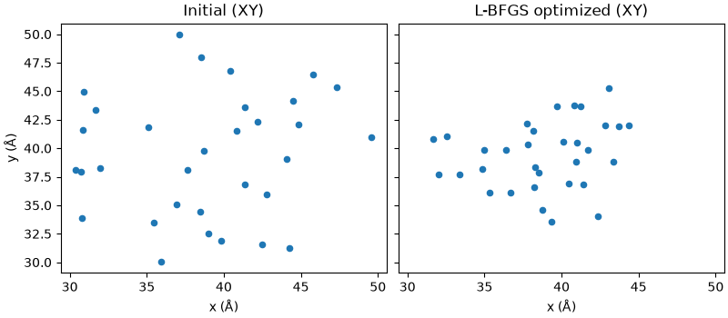
Visualize initial vs final geometry (XY projection)

fig2, ax2 = plt.subplots(
    1, 2, figsize=(8.0, 3.5), sharex=True, sharey=True, constrained_layout=True
)
ax2[0].scatter(initial_positions[:, 0], initial_positions[:, 1], s=20)
ax2[0].set_title("Initial (XY)")
ax2[0].set_xlabel("x (Å)")
ax2[0].set_ylabel("y (Å)")
ax2[1].scatter(lbfgs_positions[:, 0], lbfgs_positions[:, 1], s=20)
ax2[1].set_title("L-BFGS optimized (XY)")
ax2[1].set_xlabel("x (Å)")

plt.show()