Introducing PhysicsNeMo-Mesh: GPU-Accelerated Mesh Processing for Scientific ML
PhysicsNeMo-Mesh is a GPU-accelerated mesh processing module, built on PyTorch and TensorDict, and included in the open-source PhysicsNeMo library. It provides a) a GPU-native, high-performance mesh data structure with design choices that are particularly well-suited for ML workflows, and b) a diverse suite of accelerated mesh operations that can be used to bridge existing gaps between data preprocessing and training/inference.
Its native data format allows loading meshes from disk much more quickly than VTU (9x-88x faster in our testing; hardware-dependent) while preserving the full mesh structure that flat tensor formats like zarr typically discard. This gives you the speed you need for training while retaining the geometric and physical context needed for model- and dataset-agnostic workflows. In this post, we'll show what PhysicsNeMo-Mesh can do for your training pipeline.
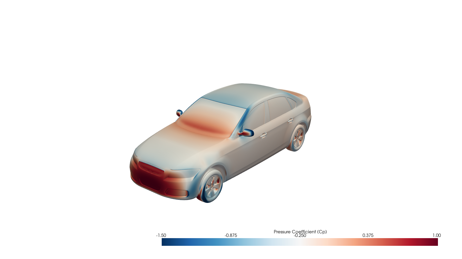 Fig 1: Surface pressure coefficient (Cp) on an 8.8 million-cell DrivAerML automotive mesh, loaded and rendered with PhysicsNeMo-Mesh.
The Data Loading Problem
Most ML training workflows that use large-scale (terabyte- to petabyte-scale) datasets from physics simulations follow four stages:
- Data generation - run simulations and serialize results in solver-native or visualizer-native formats (in fluid dynamics applications, often VTU/VTP for unstructured meshes).
- Data preprocessing - prepare data for the specific downstream ML model. This is often both model-specific and dataset-specific: computing derived quantities (SDF values, surface normals), nondimensionalization, data augmentation (e.g., random rotations to approximate rotational equivariance), and converting the data into the model's expected input format. For equivariant models, this means explicitly tagging which fields are scalars vs. vectors. For non-equivariant models, it often means concatenating all fields into a single feature tensor (
tensor[:, 0]is density,tensor[:, 1:4]is velocity, and so on) - fine for non-equivariant architectures, but it destroys the information that equivariant ones need. - Serialization for training - re-serialize the preprocessed data into a fast-loading format (NumPy
.npy/.npz, zarr, etc.), because solver-native formats like VTU are too slow for training-time loading. VTU requires CPU-bound XML parsing that takes tens of seconds to minutes per sample, and with typical Physics-AI forward and backward passes running in 0.1-10 seconds, the data loader easily becomes the bottleneck. - Training - load the serialized data and train the model.
Notice that preprocessing (step 2) happens before serialization (step 3), and training (step 4) happens after - so preprocessing and training are separated by a serialization/deserialization boundary. This means the on-disk dataset is typically tightly coupled to one model architecture and one preprocessing recipe. If you want to change the model, switch to a different dataset, do feature engineering, normalize in a different way, or do data augmentation, you likely need to re-run steps 2-3 across the entire dataset. And because flat array formats like zarr discard mesh structure - cell connectivity, topology, boundary faces, hierarchical data, the distinction between point-centered and cell-centered data - there's no going back: you can't re-derive what was lost from the serialized format.
PhysicsNeMo-Mesh provides a GPU-native Mesh data structure and associated processing tools, which ultimately give you the option of inverting the order of steps 2 and 3:
- Conventional: Generate → Preprocess → Serialize → Train
- With PhysicsNeMo-Mesh: Generate → Serialize → Preprocess → Train
In this paradigm, you serialize first - from VTU to PhysicsNeMo-Mesh's native Mesh format (*.pmsh) - and preprocess later on-the-fly at load time (i.e., as part of training or inference). This is practical because PMSH preserves the mesh structure (so all preprocessing operations remain available after deserialization), and GPU-accelerated processing makes those operations fast enough to run at training time rather than as a batch preprocessing step (up to three orders of magnitude faster than CPU-based VTK operations, in part because the simplicial mesh representation makes algorithms much easier to vectorize on the GPU).
Preprocessing and the training forward pass are now adjacent in the pipeline. Since both run on GPU, they can be fused into the same process - even within the same computational graph, with autograd flowing through both.
The immediate benefit is faster loading and higher throughput. The longer-term benefit is that by flipping the order, the serialized format becomes model- and dataset-agnostic. The same PMSH files can serve any downstream model - equivariant or non-equivariant, point-cloud-based or graph-based. This matters because model architectures are evolving quickly (re-preprocessing a derived dataset for each new architecture doesn't scale), and as research focus shifts toward generalization of ML surrogates for PDEs, multi-dataset training becomes more compelling - which requires on-disk formats that aren't locked to a single model's preprocessing assumptions. The result is a fusion of what were previously disjoint preprocessing and training stages, enabling faster iteration on model architecture development, training, and benchmarking.
Faster Loading, Smaller Files, Shorter Training
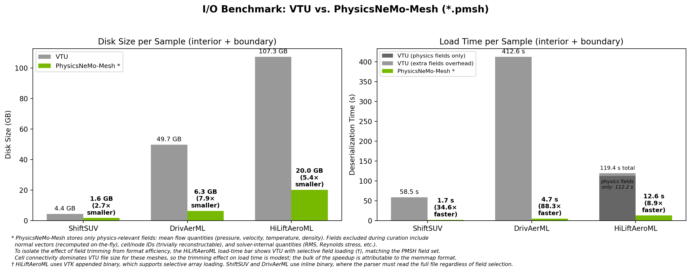 Fig 2: I/O benchmark comparing VTU and PhysicsNeMo-Mesh (*.pmsh) across three production datasets. PMSH loads are 9x-88x faster with 3-8x smaller files on disk.
The most important immediate benefit of PhysicsNeMo-Mesh-based datapipes over raw VTU/VTP formats is faster loading. The speedups are striking: on ShiftSUV, a mesh that takes 58.5 seconds to load from VTU loads in 1.7 seconds from PMSH (~35x faster). On DrivAerML, 413 seconds becomes 4.7 seconds (88x faster). Even HiLiftAeroML - 107 GB of VTU data per sample - loads in 12.6 seconds from PMSH (8.9x faster).
This speedup comes from two places. The first is that you can drop fields that are typically not needed for downstream training. For example, while many CAE datasets save surface normals, with a GPU-accelerated mesh module it is often far faster to recompute these on-the-fly rather than incur the I/O overhead of loading them from disk. Other dropped fields include cell and node IDs (trivially reconstructable) and solver-internal quantities that are not typically direct engineering quantities of interest (e.g., full Reynolds stress tensor). This field trimming, while helpful, is responsible for a surprisingly small fraction of the speedup - around 5-10% on HiLiftAeroML, as shown in the figure above. (Unlike the other two tested datasets, the HiLiftAeroML dataset uses uncompressed VTU files; these allow for selective field loading, facilitating an apples-to-apples comparison.)
The far more significant speedup comes from PhysicsNeMo-Mesh's ability to use memory-mapped (memmap) I/O via TensorDict. With this, there is near-zero parsing overhead - the mesh can be loaded byte-for-byte into memory, and the limiting factor typically becomes hard disk read bandwidth. Even after correcting for field trimming, this memmap approach is responsible for around an 8.9x speedup on HiLiftAeroML load speeds in our testing.
PhysicsNeMo-Mesh also has disk space advantages over VTU, with a 3-8x reduction in per-sample storage (as shown in Fig 2). As modern CAE simulation datasets scale to tens or hundreds of terabytes of VTU data, this disk savings can be the deciding factor in whether training on a given dataset is feasible. As with the load speed improvements, the savings come from two sources: storing data as compact binary arrays rather than VTU's XML-based encoding, and trimming of extraneous data fields.
Because Mesh is a first-class tensor structure, preprocessing steps are CUDA kernels that can be pipelined with training - the next sample's preprocessing and data transfers run concurrently with the current sample's forward and backward passes, keeping the GPU saturated. Early experiments show up to 50% training loop speedups (highly model- and dataset-dependent), a form of pipelining that isn't available when preprocessing happens offline. This is active work; we plan to share detailed results in a future post.
Structure That ML Models Need
The standard ML pipeline for physics simulations converts each mesh element into a concatenated feature vector, flattening away geometric and semantic distinctions that physically-consistent PDE surrogates need. For example:
- Euclidean equivariance requires distinguishing scalars from vectors (and higher-rank tensors) so that predictions transform correctly under rotation and reflection. Once everything is a single feature vector, this distinction is gone.
- Boundary condition encoding requires structured, heterogeneous data: different boundary types (slip, no-slip, inlet, outlet) carry fundamentally different associated quantities, and interior and boundary points and cells carry different schemas. Flat feature vectors can't naturally represent this schema variation, with the typical result being that boundary condition data is irreversibly dropped.
- PDE information flow often requires simultaneously manipulating physical fields (velocity, pressure) and nonphysical ones (network-internal latent fields), which demands a way to attach semantics to different parts of the internal representation.
PhysicsNeMo-Mesh addresses all three. The mesh is a first-class, GPU-native, autograd-compatible data structure that carries arbitrary-rank tensor fields (scalars, vectors, stress tensors) organized in nested TensorDict containers with hierarchical, semantic keys. Cell connectivity, boundary structure, and the distinction between point-centered and cell-centered data are all preserved throughout the pipeline. PhysicsNeMo-Mesh operates on simplicial meshes (triangles, tetrahedra, and their lower/higher-dimensional analogues) - see the User Guide for details on mesh types and the underlying data model.
GPU-Accelerated Mesh Processing
Beyond I/O, PhysicsNeMo-Mesh accelerates the mesh operations themselves. Common operations - computing normals, curvature, gradients, neighbor queries, subdivision - that take seconds on CPU with conventional libraries can run orders of magnitude faster on GPU:
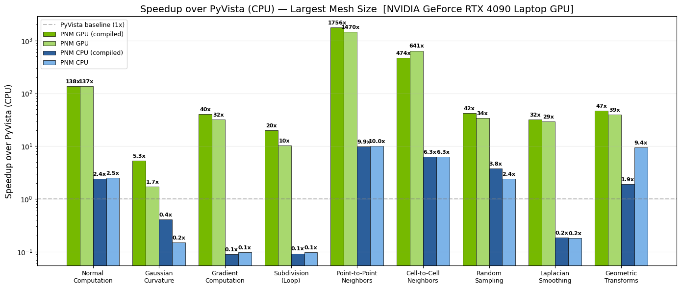 Fig 3: GPU speedup of PhysicsNeMo-Mesh over PyVista (CPU) across common mesh operations, benchmarked on an NVIDIA GeForce RTX 4090 Laptop GPU. Green bars show GPU performance; blue bars show CPU performance within PhysicsNeMo-Mesh. Darker shades indicate torch.compiled variants.
What's Available
PhysicsNeMo-Mesh is a comprehensive mesh processing module. For full details and worked examples, see the tutorial notebooks.
- Discrete calculus - gradient, divergence, curl, and Laplacian operators via DEC and least-squares methods
- Differential geometry - Gaussian and mean curvature, cell/point normals, tangent spaces
- Subdivision & remeshing - linear, Loop, and Butterfly subdivision; uniform remeshing via ACVD
- Repair - duplicate removal, degenerate cell removal, hole filling, orientation fixing
- Spatial queries - BVH-accelerated point containment, nearest-cell search, barycentric interpolation
- Topology - point/cell adjacency, boundary detection, facet extraction, manifold checking
- I/O & visualization - bidirectional PyVista conversion (STL, VTK, PLY, OBJ); PyVista/VTK rendering; matplotlib fallback
From Meshes to Graphs and Point Clouds
A graph is just a 1D mesh: nodes are mesh points, edges are mesh cells (line segments). PhysicsNeMo-Mesh provides direct conversion methods:
from physicsnemo.mesh.remeshing import remesh

car_coarse = remesh(car_mesh, n_clusters=5000)
edge_graph = car_coarse.to_edge_graph()     # vertex-centered graph
centroid_graph = car_coarse.to_dual_graph()  # cell-centered graph
point_cloud = car_mesh.to_point_cloud()      # 0D mesh, no connectivity
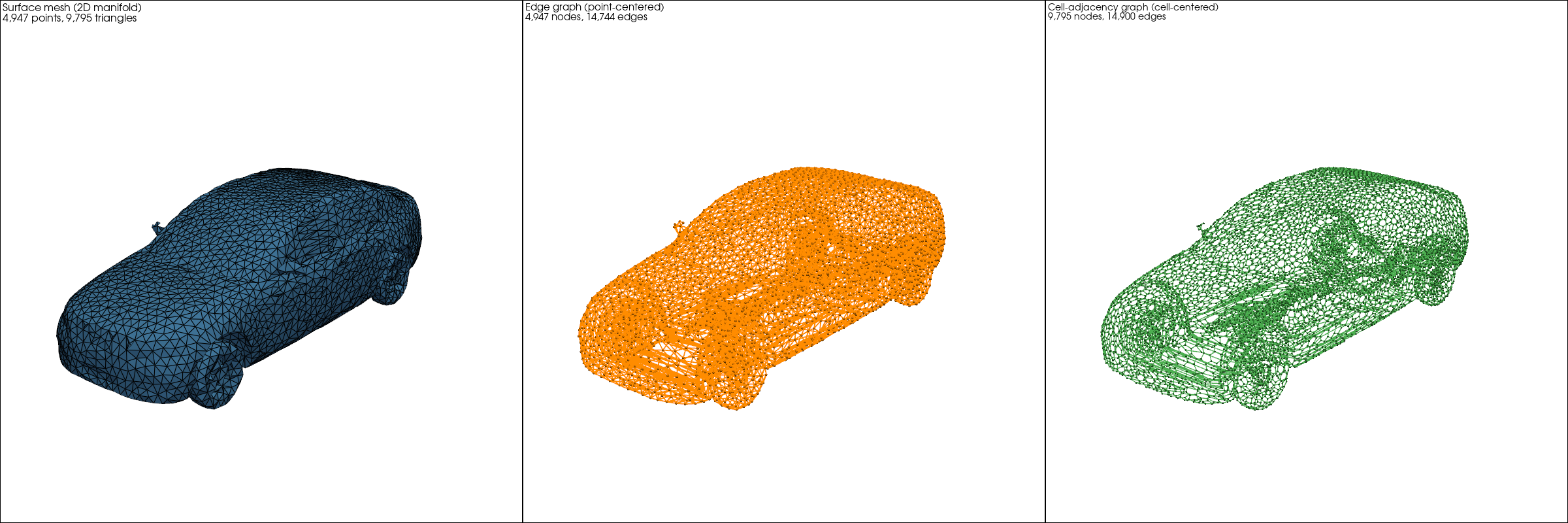 Fig 4: Three views of a DrivAerML car: the surface mesh (left), its edge graph for point-centered data (center), and its cell-adjacency graph for cell-centered data (right). All three are first-class Mesh objects.
The edge graph is natural when data lives on vertices. For cell-centered data - common in finite volume CFD - the dual graph places nodes at cell centroids with edges between adjacent cells, avoiding lossy interpolation from cells to vertices. The dual-graph edges correspond exactly to the faces where fluxes are exchanged between neighboring control volumes, making it a natural representation for finite volume formulations.
Meshes are a strict superset of graphs: they add geometric structure (areas, normals, curvature), discrete calculus operators, spatial queries, and topological operations that graph-only frameworks like PyG and DGL don't natively provide. For tasks that purely rely on abstract graphs, those frameworks remain excellent choices; PhysicsNeMo-Mesh's value is in the geometric and topological operations that become available when you retain the full mesh structure.
Computing Derived Quantities
The real power of keeping mesh structure in the training loop is computing new quantities from simulation data. Consider the DrivAerML dataset: the simulation outputs include surface pressure and wall shear stress, but we can derive the streamwise pressure gradient dp/ds - the classic indicator of boundary layer stability - by projecting the surface pressure gradient onto the local flow direction:
from physicsnemo.mesh.io import from_pyvista
import pyvista as pv

mesh = from_pyvista(pv.read("boundary_1.vtp"))
mesh = mesh.cell_data_to_point_data()
mesh = mesh.compute_point_derivatives(keys="pMeanTrim", gradient_type="extrinsic")

grad_p = mesh.point_data["pMeanTrim_gradient"]          # (n_points, 3)
wss = mesh.point_data["wallShearStressMeanTrim"]         # (n_points, 3)
wss_hat = wss / wss.norm(dim=-1, keepdim=True).clamp(min=1e-8)
mesh.point_data["adverse_pg"] = (grad_p * wss_hat).sum(dim=-1)
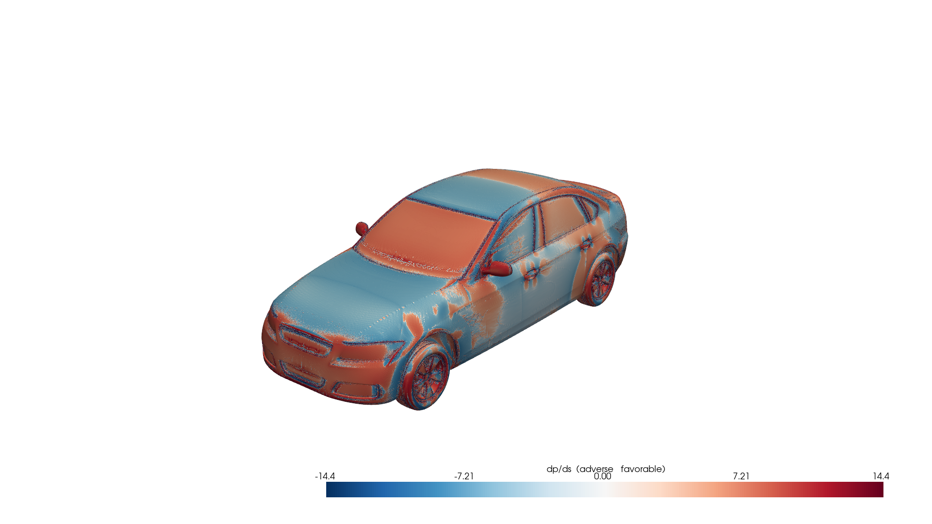 Fig 5: Adverse pressure gradient indicator on the DrivAerML car. Red regions indicate adverse pressure gradients (destabilizing), blue regions indicate favorable gradients (stabilizing). Computed from raw CFD data using PhysicsNeMo-Mesh gradient operators.
This workflow - loading simulation data, converting between cell and point representations, computing surface gradients, combining fields - is representative of the feature engineering that PhysicsNeMo-Mesh makes straightforward. Each step is GPU-accelerated and autograd-compatible - and because these operations happen at training time rather than as a batch preprocessing step, changing your feature engineering recipe means changing code, not re-processing the entire dataset.
Case Study: GLOBE - A Neural Surrogate Built on Mesh
A powerful illustration of what becomes possible when your ML architecture is built on a proper mesh module is the GLOBE model (Green's-function-Like Operator for Boundary Element PDEs), recently merged into PhysicsNeMo at physicsnemo.experimental.models.globe.
GLOBE is a kernel-based neural field inspired by boundary element method PDE solvers. It represents solutions as superpositions of learnable Green's-function-like kernels evaluated from boundary faces to target points. Its internal state is itself a collection of Mesh objects - the model receives boundary meshes with boundary condition data in cell_data, processes them through communication hyperlayers, and produces predictions at arbitrary query points.
Notably, GLOBE takes boundary condition information as an explicit, structured input: boundary_meshes: dict[str, Mesh], where dictionary keys identify condition types (e.g., "no_slip", "freestream") and each mesh's cell_data carries the associated values. Boundary conditions are explicit inputs to the model, not inferred from geometric heuristics or dataset-specific correlations.
Building on PhysicsNeMo-Mesh gives GLOBE:
- Structured latent state. Latent activations are stored in a nested TensorDict within
cell_data(e.g.,mesh.cell_data["latent", "scalars", "0"]), not as opaque flat tensors. GLOBE uses this separation to treat scalar channels as rotation-invariant and vector channels as covariant under rotation, supporting equivariant operations. - Discretization invariance. Area-weighted integration via
mesh.cell_areasensures predictions converge to a well-defined limit as the mesh is refined, independent of the particular discretization. - Reusable mesh utilities. Subdivision, remeshing, and interpolation are available out of the box for upscaling or downscaling between training and inference.
- Debuggability. Call
mesh.draw(cell_scalars=("latent", "scalars", "0"))at any breakpoint in the forward pass to visualize latent activations. You can trace numerical instabilities, identify dead channels, or understand what the model has learned - no custom visualization code needed, because the data already carries its own geometry.
Getting Started
PhysicsNeMo-Mesh is available now as part of PhysicsNeMo.
- Source code: physicsnemo/mesh/
- API documentation for Mesh: PhysicsNeMo Docs
- Mesh User Guide: Mesh User Guide (coming soon) - concepts, data model, and usage patterns
- Tutorial notebooks: examples/minimal/mesh/ - six Jupyter notebooks covering mesh creation, operations, discrete calculus, spatial queries, quality/repair, and ML integration
- GLOBE model: physicsnemo.experimental.models.globe
Install with:
pip install "nvidia-physicsnemo[cu13,mesh-extras]"
We're excited to see what you build with PhysicsNeMo-Mesh. If you have questions or feedback, visit our GitHub Discussions.