Time Series Forecasting#

Time series foundation models (TSFMs) predict future values of a series from its observed history. While many forecasting foundation models originally focused on predicting a single variable from its own history (univariate forecasting), newer models such as Chronos-2 and TimesFM-3 extend this paradigm to multiple targets (multivariate forecasting) and covariates: additional variables that inform the forecast (e.g., historical temperature or planned promotions). These capabilities allow models to draw on relationships between targets, past observations of external factors, and known future information.

Time series forecasting shares a central principle with tabular in-context learning: a pretrained model conditions its predictions on observed examples, without requiring training on each new dataset. In tabular prediction, the context consists of labeled rows and the queries are new rows. In forecasting, the context is the observed past and the queries are future time steps. In both settings, attention across columns captures relationships between variables within a row or time step, while attention across rows captures relationships between observations or time steps. Forecasting thus motivates useful extensions to the in-context learning formulation:

Multiple targets allow a model to predict several variables together.
Known future covariates provide inputs for both context and query rows.
Past-only covariates provide inputs for context rows even when their query values are unavailable.

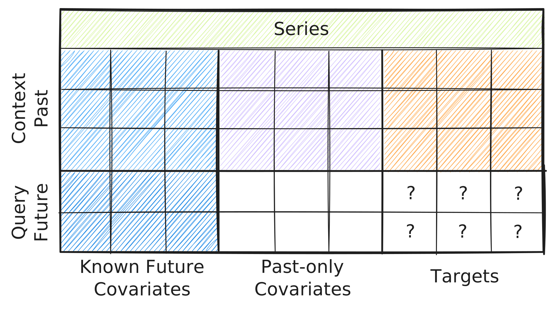
This package incorporates these extensions through the same ICLModel used by other models. In particular, y_context contains the observed targets, columns shared by x_context and x_query represent known future covariates, and columns exclusive to x_context represent past-only covariates.

Univariate Forecasting#

We begin with a single target, the daily sales of ice cream, observed for five days and forecast for the next three:

day	0	1	2	3	4	5	6	7
ice cream	40	55	80	75	50	?	?	?

We represent a time series as a TableTensor with one row per time step, sorted in time, and one column per variable:

import sdm

history = sdm.TableTensor.from_columns(
    {"ice_cream": [40.0, 55.0, 80.0, 75.0, 50.0]},
    stypes={"ice_cream": "numerical"},
    device="cuda",
)

We can forecast with any time series forecasting model in sdm.models. Here, we use Chronos2:

model = sdm.models.Chronos2(device="cuda")
out = model(
    x_context=sdm.TableTensor(size=(5, ), device="cuda"),
    y_context=history,
    x_query=sdm.TableTensor(size=(3, ), device="cuda"),
)

Note that x_context and x_query carry the covariates. Since we have none yet, both tables hold zero columns. However, we still need to pass them to forward(), in particular because the number of rows in x_query defines the forecast horizon: here, we request predictions for the next three time steps.

The forecast is returned as a TableTensor with one row per future step. Its output is model-specific, e.g., Chronos2 outputs one column per target and quantile, named "<target>__q<level>":

out["ice_cream__q50"].numerical  # median forecast, [3, 1]
out["ice_cream__q10"].numerical  # lower end of an 80% prediction interval
out["ice_cream__q90"].numerical  # upper end of an 80% prediction interval

Multivariate Forecasting#

A model that supports_multi_target can forecast multiple targets jointly, allowing them to exploit dependencies between them.

In this case, we can simply add the daily sales of cold drinks as a second target:

day	0	1	2	3	4	5	6	7
ice cream	40	55	80	75	50	?	?	?
cold drinks	25	30	45	41	28	?	?	?

history = sdm.TableTensor.from_columns(
    {
        "ice_cream": [40.0, 55.0, 80.0, 75.0, 50.0],
        "cold_drinks": [25.0, 30.0, 45.0, 41.0, 28.0],
    },
    stypes={"ice_cream": "numerical", "cold_drinks": "numerical"},
    device="cuda",
)

out = model(
    x_context=sdm.TableTensor(size=(5, ), device="cuda"),
    y_context=history,
    x_query=sdm.TableTensor(size=(3, ), device="cuda"),
)

Covariates#

Lastly, we add known future and past-only covariates to our model. For example, the measured temperature is a past-only covariate: its values are unavailable for the forecast horizon. A model that supports_context_only_columns can exploit such past-only covariates. In contrast, promotion is a known future covariate that indicates whether a promotion was or is scheduled for a given day.

day	0	1	2	3	4	5	6	7
ice cream	40	55	80	75	50	?	?	?
cold drinks	25	30	45	41	28	?	?	?
temperature	21	24	28	27	22
promotion	0	0	1	1	0	1	0	0

history = sdm.TableTensor.from_columns(
    {
        "ice_cream": [40.0, 55.0, 80.0, 75.0, 50.0],
        "cold_drinks": [25.0, 30.0, 45.0, 41.0, 28.0],
        "temperature": [21.0, 24.0, 28.0, 27.0, 22.0],
        "promotion": [0.0, 0.0, 1.0, 1.0, 0.0],
    },
    stypes={
        "ice_cream": "numerical",
        "cold_drinks": "numerical",
        "temperature": "numerical",
        "promotion": "numerical",
    },
    device="cuda",
)
future = sdm.TableTensor.from_columns(
    {"promotion": [1.0, 0.0, 0.0]},
    stypes={"promotion": "numerical"},
    device="cuda",
)

out = model(
    x_context=history[["temperature", "promotion"]],
    y_context=history[["ice_cream", "cold_drinks"]],
    x_query=future,
)

In summary, the columns that are passed determine which covariates the model sees:

Known future covariates appear in both x_context and x_query.
Past-only covariates appear in x_context only.
Without any covariates, x_context and x_query have zero columns.

Ensembling#

As with any other ICLModel, the num_estimators argument controls how many ensemble members contribute to the forecast. Each member may receive a differently transformed view of the series, and their predictions are averaged into a single forecast. For example, the default recipe for TimesFM3 alternates between the original series and a sign-flipped version. Using two estimators includes both views:

out = model(x_context, y_context, x_query, num_estimators=2)

Batched Forecasting#

Batching lets us run several independent forecasting tasks in one call. Each task has its own context and queries, and predictions will not use information from other tasks in the batch. Each task itself can contain multiple targets and covariates.

For example, store sales can be represented in two ways: as separate univariate tasks in a batch (forecasting each store independently) or as a multivariate task (allowing the model to use relationships between stores).

To forecast a batch of series in one call, stack them along a leading batch dimension. All series in a batch share the same horizon and number of context rows, and shorter series should be left-padded with NaN. Set num_estimators explicitly so that the leading dimension is interpreted as a batch of independent forecasting tasks rather than as ensemble members:

import torch

out = model(
    x_context=torch.randn(64, 128, 0, device="cuda"),
    y_context=torch.randn(64, 128, 2, device="cuda"),
    x_query=torch.randn(64, 32, 0, device="cuda"),
    num_estimators=1,
)

See examples/timeseries/forecast.py for runnable examples on real-world datasets and tasks.