Speech Commands
Introduction
The ability to recognize spoken commands with high accuracy can be useful in a variety of contexts. To this end, Google recently released the Speech Commands dataset (see paper), which contains short audio clips of a fixed number of command words such as “stop”, “go”, “up”, “down”, etc spoken by a large number of speakers. To promote the use of the set, Google also hosted a Kaggle competition, in which the winning team attained a multiclass accuracy of 91%.
We experimented with applying OpenSeq2Seq’s existing image classification models on mel spectrograms of the audio clips and found that they worked surprisingly well. Adding data augmentation further improved the results.
Dataset
Google released two versions of the dataset with the first version containing 65k samples over 30 classes and the second containing 110k samples over 35 classes. However, the Kaggle contest specification used only 10 of the provided classes, grouped the others as “unknown” and added “silence” for a total of 12 labels. We refer to these datasets as v1-12, v1-30 and v2, and have separate metrics for each version in order to compare to the different metrics used by other papers.
To preprocess a given version, we run speech_commands_preprocessing.py which first separates each class into training, validation and test sets with an 80-10-10 split. The script then balances the number of samples in each class by randomly duplicating samples in each class, which effectively grows the dataset since we apply random transformations to each sample in the data layer.
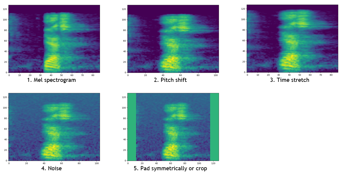
These samples are fed into the data layer, which randomly pitch shifts, time stretches and adds noise to each audio sample. These augmented samples are then converted into mel spectrograms and either randomly sliced or symmetrically padded with zeros until they are fixed dimension and square. These transformations are shown below.
To solve the bounded host bottleneck, the transformed images are cached during the first epoch in order to increase GPU utilization on subsequent epochs.
Models
The output of the data layer is a square image (128x128), which can then be fed into either ResNet or Jasper.
ResNet-50
The configuration file used for ResNet can be found here. The models were trained in mixed precision on 8 GPUs with a batch size of 32 over 100 epochs.
| Dataset | Validation Accuracy | Test Accuracy | Checkpoint |
|---|---|---|---|
| v1-12 | 96.6% | 96.6% | link |
| v1-30 | 97.5% | 97.3% | link |
| v2 | 95.7% | 95.9% | link |
Jasper-10x3
The configuration file used for Jasper can be found here. The models were trained in mixed precision on 8 GPUs with a batch size of 64 over 200 epochs.
| Dataset | Validation Accuracy | Test Accuracy | Checkpoint |
|---|---|---|---|
| v1-12 | 97.1% | 96.2% | link |
| v1-30 | 97.5% | 97.3% | link |
| v2 | 95.5% | 95.1% | link |
To use a different dataset, the only change required is to the dataset_version parameter, which should be set to one of v1-12, v1-30 or v2.
Mixed Precision
We found that the model trains just as well in mixed precision, attaining the same results with half the GPU memory. A constant loss scaling of 512.0 was used for ResNet, which saw a 12% speedup from float using the same batch size. Similarly, backoff loss scaling was used for Jasper, which saw a 15% speedup from float.
