Deutschs’ Algorithm

We have a function which takes in a bit and outputs a bit. This can be represented as \(f: \{0,1\} \longrightarrow \{0,1\}\).

The function \(f\) has a property; either it is constant or balanced.

If constant, the outputs are the same regardless of the inputs i.e. \(f(0) = f(1) = 0\) or \(f(0) = f(1) = 1\).

If balanced, the ouputs are balanced across their possibilities, i.e, if \(f(0) = 0\) then \(f(1) = 1\) or if \(f(0) = 1\) then \(f(1) = 0\).

The question we would like to answer is if the function is constant or balanced.

Classically, if we are given a function \(f\), we can solve to find its property via the code below:

# Treat the code snippet below like a black box, i.e you dont have access to the value of the property argument and can just query f with different inputs.


def f(x, property='constant'):

    if property == 'constant':

        # The output is a 1 regardless of the input, we can also make the output to be 0.

        if x == 0:
            return 1
        elif x == 1:
            return 1

    if property == 'balanced':

        # The output depends on the input.

        if x == 0:
            return 1
        elif x == 1:
            return 0

Let us now classically find out if the function we defined above is constant or balanced.

if f(0) == 0:
    if f(1) == 0:
        print('The function is constant')
    elif f(1) == 1:
        print('The function is balanced')

elif f(0) == 1:
    if f(1) == 1:
        print('The function is constant')
    elif f(1) == 0:
        print('The function is balanced')

The function is constant

If you step through the if statements above, one can see that we require 2 calls to the function to determine its property. That is we have to query \(f\) twice.

The claim is that Deutschs’ algorithm can solve for this property with 1 function evalulation demonstrating quantum advantage.

Below we first go through the math and then the implementation in CUDA Quantum.

XOR \(\oplus\)

You may have seen the \(\oplus\) symbol floating around. This is the exclusive OR or the XOR operation. It follows the rules of addition modulo 2. For example,

1. \(3\oplus5 = (3+5)_{\%2} = 8_{\%2} = 0\)

2. \(5\oplus4 = (5+4)_{\%2} = 9_{\%2} = 1\)

A quick way to perform the \(\oplus\) calculation is if the result of the addition is an even number, the result is 0 otherwise 1.

Quantum oracles

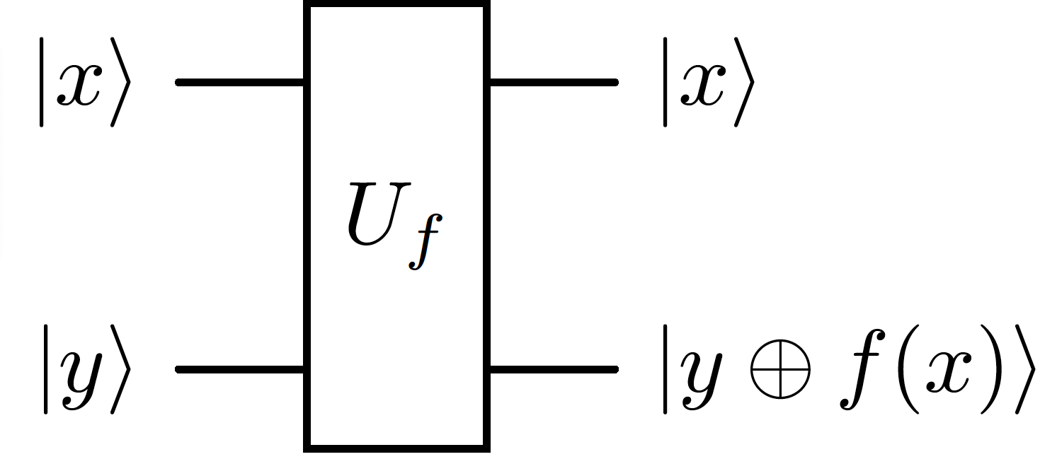
Suppose we have \(f(x): \{0,1\} \longrightarrow \{0,1\}\). We can compute this function on a quantum computer using oracles which we treat as black box functions that yield the output with an appropriate sequence of logic gates.

Above you see an oracle represented as \(U_f\) which allows us to transform the state \(\ket{x}\ket{y}\) into:

\[\begin{aligned} U_f\ket{x}\ket{y} = \ket{x}\ket{y \oplus f(x)} \end{aligned}\]

If \(y = 0\), then \(U_f\ket{x}\ket{y} = U_f\ket{x}\ket{0} = \ket{x}\ket{0 \oplus f(x)} = \ket{x}\ket{f(x)}\) since \(f(x)\) can either be \(0/1\) and \(0 \oplus 0 = 0\) and \(0 \oplus 1 = 1\).

This is remarkable as by setting \(\ket{y} = \ket{0}\), we can extract the value of \(f(x)\) by measuring the value of the second qubit.

Phase oracle

Since \(f(x)\) can be either \(0/1\), \(0 \oplus f(x) = 0 \oplus 0/1 = 0/1 = f(x)\).

Similarly, \(1 \oplus f(x) = 1 \oplus 0/1 = 1/0 = \overline{f(x)}\) where the bar on top of \(f(x)\) denotes ‘not \(f(x)\)’.

Let us now prove a result which we shall use later:

\[\begin{split}\begin{aligned} U_f\ket{x}\ket{-} &= U_f \ket{x} \tfrac{1}{\sqrt{2}}(\ket{0} - \ket{1}) \\ &= \tfrac{1}{\sqrt{2}} (U_f\ket{x}\ket{0} - U_f\ket{x}\ket{1}) \\ &= \tfrac{1}{\sqrt{2}} (\ket{x}\ket{0 \oplus f(x)} - \ket{x}\ket{1 \oplus f(x)}) \\ &= \tfrac{1}{\sqrt{2}} (\ket{x}\ket{f(x)} - \ket{x}\ket{\overline{f(x)}}) \\ &= \begin{cases} \tfrac{1}{\sqrt{2}} (\ket{x}\ket{0} - \ket{x}\ket{1}) = \ket{x}\ket{-} & f(x) = 0 \\ \tfrac{1}{\sqrt{2}} (\ket{x}\ket{1} - \ket{x}\ket{0}) = -\ket{x}\ket{-} & f(x) = 1 \\ \end{cases} \\ &= (-1)^{f(x)}\ket{x}\ket{-} \end{aligned}\end{split}\]

In summary, \(U_f\ket{x}\ket{-} = (-1)^{f(x)}\ket{x}\ket{-}\) where the \(\ket{-}\) qubit was left unchanged and a phase was applied to \(\ket{x}\)

Quantum parallelism

Consider:

\[\begin{split}\begin{aligned} U_f\ket{+}\ket{0} &= U_f \tfrac{1}{\sqrt{2}}(\ket{0}+\ket{1}) \ket{0} \\ &= U_f \tfrac{1}{\sqrt{2}}(\ket{0}\ket{0}+\ket{1}\ket{0}) \\ &= \tfrac{1}{\sqrt{2}}(U_f \ket{0}\ket{0} + U_f \ket{1}\ket{0}) \\ &= \tfrac{1}{\sqrt{2}}(U_f \ket{0}\ket{0} + U_f \ket{1}\ket{0}) \\ &= \tfrac{1}{\sqrt{2}}(\ket{0}\ket{0 \oplus f(0)} + \ket{1}\ket{0 \oplus f(1)}) \\ &= \tfrac{1}{\sqrt{2}}(\ket{0}\ket{f(0)} + \ket{1}\ket{f(1)}) \\ \end{aligned}\end{split}\]

We have calculated information about both \(f(0)\) and \(f(1)\) simultaneously. Quantum mechanics allows for parallelism by exploiting the ability of superposition states.

Deutschs’ Algorithm:

Our aim is to find out if \(f: \{0,1\} \longrightarrow \{0,1\}\) is a constant or a balanced function? If constant, \(f(0) = f(1)\), and if balanced, \(f(0) \neq f(1)\).

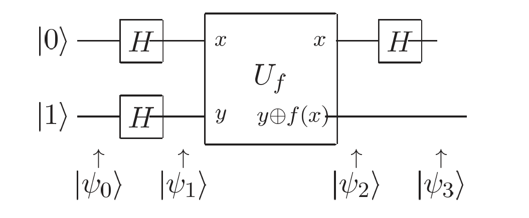
We step through the circuit diagram below and follow the math after the application of each gate.

\[\ket{\psi_0} = \ket{01} \tag{1}\]

\[\ket{\psi_1} = H_1H_0\ket{\psi_0} = H_1H_0\ket{01} = \ket{+-} = \frac{1}{\sqrt{2}} (\ket{0}+\ket{1})\ket{-} \tag{2}\]

\[\ket{\psi_2} = U_f\ket{\psi_1} = \frac{1}{\sqrt{2}} (U_f\ket{0}\ket{-} + U_f\ket{1}\ket{-}) \tag{3}\]

using \(U_f\ket{x}\ket{-} = (-1)^{f(x)}\ket{x}\ket{-}\) which we proved in the phase oracle section above:

\[\begin{split}\begin{aligned} \ket{\psi_2} = \frac{1}{\sqrt{2}} ((-1)^{f(0)}\ket{0}\ket{-} + (-1)^{f(1)}\ket{1}\ket{-}) \\ = \frac{1}{\sqrt{2}} ((-1)^{f(0)}\ket{0} + (-1)^{f(1)}\ket{1}) \ket{-} \\ \end{aligned}\end{split}\]

We now drop the second, qubit in the \(\ket{-}\) state from our derivations as the figure above has no further gate operations acting on it. Remember our aim is to find out if \(f(x)\) is a constant or a balanced function. We have the following options:

\[\begin{split}\begin{aligned} \ket{\psi_{2}}= \begin{cases} \tfrac{1}{\sqrt{2}} (\ket{0} + \ket{1}) & f(0) = 0, f(1) = 0, f(x) \text{ is constant} \\ -\tfrac{1}{\sqrt{2}} (\ket{0} + \ket{1}) & f(0) = 1, f(1) = 1, f(x) \text{ is constant} \\ \tfrac{1}{\sqrt{2}} (\ket{0} - \ket{1}) & f(0) = 0, f(1) = 1, f(x) \text{ is balanced} \\ -\tfrac{1}{\sqrt{2}} (\ket{0} - \ket{1}) & f(0) = 1, f(1) = 0, f(x) \text{ is balanced} \\ \end{cases} \end{aligned}\end{split}\]

\[\begin{split}\begin{aligned} \ket{\psi_{2}} = \begin{cases} \pm \tfrac{1}{\sqrt{2}} (\ket{0} + \ket{1}) = \pm \ket{+} & f(x) \text{ is constant} \\ \pm \tfrac{1}{\sqrt{2}} (\ket{0} - \ket{1})= \pm \ket{-} & f(x) \text{ is balanced} \\ \end{cases} \end{aligned}\end{split}\]

\[\begin{split}\begin{aligned} \ket{\psi_{3}}= H\ket{\psi_{2}} \begin{cases} \pm H\ket{+} = \pm \ket{0} & f(x) \text{ is constant} \\ \pm H\ket{-} = \pm \ket{1} & f(x) \text{ is balanced} \\ \end{cases} \end{aligned}\end{split}\]

We can now measure the first qubit to yield either a \(0/1\) to determine if \(f(x)\) is constant or balanced.

Deutschs’ algorithm may not be practically useful but does demonstrate quantum advantage since it uses one function call to determine the property of \(f\) in comparison to two for classical methods.

# Import the CUDA-Q package and set the target to run on NVIDIA GPUs.

import cudaq
import numpy as np

from typing import List

cudaq.set_target("nvidia")

# Here we input the values of [f(0), f(1)] which allows us to represent constant or balanced functions.

fx = [0, 1]

# Let us now code up the circuit shown above following the state Psi after each step.

qubit_count = 2


@cudaq.kernel
def kernel(fx: List[int]):
    qubit_0 = cudaq.qubit()
    qubit_1 = cudaq.qubit()

    # Psi 0
    x(qubit_1)

    # Psi 1
    h(qubit_0)
    h(qubit_1)

    # Psi 2 - oracle
    if fx[0] == 1:
        x.ctrl(qubit_0, qubit_1)
        x(qubit_1)

    if fx[1] == 1:
        x.ctrl(qubit_0, qubit_1)

    # Psi 3
    h(qubit_0)

    # Measure the qubit to yield if the function is constant or balanced.
    mz(qubit_0)


print(cudaq.draw(kernel, fx))

result = cudaq.sample(kernel, fx, shots_count=1)

if np.array(result)[0] == '0':
    print('f(x) is a constant function')
elif np.array(result)[0] == '1':
    print('f(x) is a balanced function')

     ╭───╮          ╭───╮
q0 : ┤ h ├───────●──┤ h ├
     ├───┤╭───╮╭─┴─╮╰───╯
q1 : ┤ x ├┤ h ├┤ x ├─────
     ╰───╯╰───╯╰───╯

f(x) is a balanced function