Note
Go to the end to download the full example code
Running Ensemble Inference#
The following notebook demostrates how to use Earth-2 MIP’s config schema and builtin inference workflows to perform ensemmble inference of the FourCastNetv2 small (FCNv2-sm) weather model with an intial state pulled from the Climate Data Store (CDS) and perturbed with random noise. The ensemble output will then be loaded into an Xarray Dataset and some sample data analysis is provided.
In summary this notebook will cover the following topics:
Configuring and setting up FCNv2 model registry
An ensemble configuration file
Running ensemble inference in Earth-2 MIP to produce an xarray DataSet
Post processing results
Set Up#
Starting off with imports, hopefully you have already installed Earth-2 MIP from this repository. There are a few additional packages needed.
import json
import os
Prior to importing Earth-2 MIP, users need to be aware of a few enviroment variables which can be used to customize Earth-2 MIPs global behavior. These must be set prior to importing Earth-2 MIP. There are a number of different configuration options, some to consider are:
WORLD_SIZE: Tells Earth-2 MIP (which uses Modulus under the hood) the number of GPUs to use for inferencing.
MODEL_REGISTRY: This variable tells Earth-2 MIP where location the model registery. By default this is located in ${HOME}/.cache/earth2mip/models.
Key Concept: A model registry is a folder that Earth-2 MIP will explore to find model checkpoints to load. A folder containing the required fileds is referred to as a “model package”. Model packages typically consist of a few files such as:
weights.tar/weights.mdlus: the model checkpoint to load
metadata.json: a JSON file that contains meta info regarding various details for using the model
config.json: constains parameters needed to instantiate the model object in python
global_means.npy: A numpy array containing the mean values used for normalization of data in the model
global_std.npy: A numpy array containing the standard deviation values used for normalization of data in the model
import dotenv
import xarray

dotenv.load_dotenv()

# With the enviroment variables set now we import Earth-2 MIP
from earth2mip import inference_ensemble, registry
/usr/local/lib/python3.10/dist-packages/gribapi/__init__.py:23: UserWarning: ecCodes 2.31.0 or higher is recommended. You are running version 2.30.0
  warnings.warn(
The cell above created a model registry folder for us, but if this is your first notebook its likely empty. Lets fix that. As previously metioned we will be using the FCNv2-sm weather model with the checkpoint provided on the Nvidia Modulus model registry. The model is shipped via a zip folder containing the required checkpoint files discussed above.
Since this model is built into Earth-2 MIP, the registry.get_model function can be used to auto-download and extract it (this can take a bit). The e2mip:// prefix on the model URI, will point Earth-2 MIP to use the package fetch methods built into the model. Without it, Earth-2 MIP will simply look for a fcnv2_sm folder in your model registry and not attempt to download anything for you. Once complete, go look in your MODEL_REGISTRY folder and the files needed for FCNv2 should now be present.
print("Fetching model package...")
package = registry.get_model("e2mip://fcnv2_sm")
Fetching model package...
The final setup step is to set up your CDS API key so we can access ERA5 data to act as an initial state. Earth-2 MIP supports a number of different initial state data sources that are supported including HDF5, CDS, GFS, etc. The CDS initial state provides a convenient way to access a limited amount of historical weather data. Its recommended for accessing an initial state, but larger data requirements should use locally stored weather datasets.
Enter your CDS API uid and key below (found under your profile page). If you don’t a CDS API key, find out more here.
cds_api = os.path.join(os.path.expanduser("~"), ".cdsapirc")
if not os.path.exists(cds_api):
    uid = input("Enter in CDS UID (e.g. 123456): ")
    key = input("Enter your CDS API key (e.g. 12345678-1234-1234-1234-123456123456): ")
    # Write to config file for CDS library
    with open(cds_api, "w") as f:
        f.write("url: https://cds.climate.copernicus.eu/api/v2\n")
        f.write(f"key: {uid}:{key}\n")
Running Inference#
To run inference we will use the earth2mip/ensemble_inference.py part of Earth-2 MIP. When this Python file, we provide either a config JSON file or a JSON serialized string for it to parse. This config contains the information regarding how the model should run inference. The schema of this can be found in earth2mip/schema/EnsembleRun.
Since we are working in a notebook, lets create this config Pythonically. There are quite a few parameters that can be used, but lets focus in on a few key ones:
ensemble_members: Number ensemble members in the forecast
noise_amplitude: The amplitude of the noise pertibation method (we find that a good value to start with is 0.05, feel free to experiment)
simulation_length: Number of (6h) time-steps to predict
weather_event: This defines the weather event as a combination of an initial time and a domain.
output_path: The output location of the ensemble prediction netCDF file
weather_model: The model ID to run. This MUST match the name of the model registry folder with your checkpoint files. So for this example its fcnv2_sm.
Note
Note: While in later notebooks we will demonstrate more Pythonic methods to interact with Earth-2 MIP’s APIs, the built in inference workflows provide a high-degree of control with little to no programming.
config = {
    "ensemble_members": 4,
    "noise_amplitude": 0.05,
    "simulation_length": 10,
    "weather_event": {
        "properties": {
            "name": "Globe",
            "start_time": "2018-06-01 00:00:00",
            "initial_condition_source": "cds",
        },
        "domains": [
            {
                "name": "global",
                "type": "Window",
                "diagnostics": [{"type": "raw", "channels": ["t2m", "u10m"]}],
            }
        ],
    },
    "output_path": "outputs/01_ensemble_notebook",
    "output_frequency": 1,
    "weather_model": "fcnv2_sm",
    "seed": 12345,
    "use_cuda_graphs": False,
    "ensemble_batch_size": 1,
    "autocast_fp16": False,
    "perturbation_strategy": "correlated",
    "noise_reddening": 2.0,
}
Now we run the main() function in earth2mip.inference_ensemble providing our config object which will run inference with the following steps:
Instantiate and load the FCNv2 small weather model onto the device
Download the initial state data needed from CDS using your saved API key
Perturb the initial state based on the parameters in the config and run a forecast predicton
Save output Xarray dataset to NetCDF file located in ../outputs/01_ensemble_notebook (the process may take a while!)
# Option 1: Use config file and CLI (use this outside a notebook)
# with open('./01_config.json', 'w') as f:
#     json.dump(config, f)
# ! python3 -m earth2mip.inference_ensemble 01_config.json

# Option 2: Feed in JSON string directly into main function
config_str = json.dumps(config)
inference_ensemble.main(config_str)
INFO:root:Earth-2 MIP config loaded weather_model='fcnv2_sm' simulation_length=10 perturbation_strategy=<PerturbationStrategy.correlated: 'correlated'> perturbation_channels=None noise_reddening=2.0 noise_amplitude=0.05 output_frequency=1 output_grid=None ensemble_members=4 seed=12345 ensemble_batch_size=1 forecast_name=None weather_event=WeatherEvent(properties=WeatherEventProperties(name='Globe', start_time=datetime.datetime(2018, 6, 1, 0, 0), initial_condition_source=<InitialConditionSource.cds: 'cds'>, netcdf='', restart=''), domains=[Window(type='Window', name='global', lat_min=-90, lat_max=90, lon_min=0, lon_max=360, diagnostics=[Diagnostic(type='raw', function='', channels=['t2m', 'u10m'], nbins=10)])]) output_dir=None output_path='outputs/01_ensemble_notebook' restart_frequency=None grf_noise_alpha=2.0 grf_noise_sigma=5.0 grf_noise_tau=2.0
INFO:root:Loading model onto device cuda:0
INFO:root:Constructing initializer data source
INFO:root:Running inference
INFO:earth2mip.initial_conditions.cds:Data not found in cache. Downloading reanalysis-era5-pressure-levels to /root/.cache/earth2mip/cds/554d2477eace4300c920ab161c2fa95b0053649ab9e5c8d43eaa9f5f9b6d248c/reanalysis-era5-pressure-levels.grib
INFO:earth2mip.initial_conditions.cds:Data not found in cache. Downloading reanalysis-era5-single-levels to /root/.cache/earth2mip/cds/a4d33dfecb006b7ab66638da1c524bc2f379c7b5f2f954d904c72eeeeadfcb40/reanalysis-era5-single-levels.grib
2023-12-08 22:16:37,626 INFO Welcome to the CDS
INFO:cdsapi:Welcome to the CDS
2023-12-08 22:16:37,627 INFO Sending request to https://cds.climate.copernicus.eu/api/v2/resources/reanalysis-era5-single-levels
INFO:cdsapi:Sending request to https://cds.climate.copernicus.eu/api/v2/resources/reanalysis-era5-single-levels
2023-12-08 22:16:37,634 INFO Welcome to the CDS
INFO:cdsapi:Welcome to the CDS
2023-12-08 22:16:37,634 INFO Sending request to https://cds.climate.copernicus.eu/api/v2/resources/reanalysis-era5-pressure-levels
INFO:cdsapi:Sending request to https://cds.climate.copernicus.eu/api/v2/resources/reanalysis-era5-pressure-levels
2023-12-08 22:16:38,010 INFO Request is completed
INFO:cdsapi:Request is completed
2023-12-08 22:16:38,011 INFO Downloading https://download-0020.copernicus-climate.eu/cache-compute-0020/cache/data6/adaptor.mars.internal-1701841835.0532813-29584-5-2fb2077e-9f77-4fa3-8996-f3192ee31461.grib to /root/.cache/earth2mip/cds/a4d33dfecb006b7ab66638da1c524bc2f379c7b5f2f954d904c72eeeeadfcb40/reanalysis-era5-single-levels.grib.tmp (15.8M)
INFO:cdsapi:Downloading https://download-0020.copernicus-climate.eu/cache-compute-0020/cache/data6/adaptor.mars.internal-1701841835.0532813-29584-5-2fb2077e-9f77-4fa3-8996-f3192ee31461.grib to /root/.cache/earth2mip/cds/a4d33dfecb006b7ab66638da1c524bc2f379c7b5f2f954d904c72eeeeadfcb40/reanalysis-era5-single-levels.grib.tmp (15.8M)
2023-12-08 22:16:38,013 INFO Downloading https://download-0007-clone.copernicus-climate.eu/cache-compute-0007/cache/data9/adaptor.mars.internal-1701841835.1326218-26433-11-b73f4345-321c-46de-bf8d-9e17f6de9980.grib to /root/.cache/earth2mip/cds/554d2477eace4300c920ab161c2fa95b0053649ab9e5c8d43eaa9f5f9b6d248c/reanalysis-era5-pressure-levels.grib.tmp (128.7M)
INFO:cdsapi:Downloading https://download-0007-clone.copernicus-climate.eu/cache-compute-0007/cache/data9/adaptor.mars.internal-1701841835.1326218-26433-11-b73f4345-321c-46de-bf8d-9e17f6de9980.grib to /root/.cache/earth2mip/cds/554d2477eace4300c920ab161c2fa95b0053649ab9e5c8d43eaa9f5f9b6d248c/reanalysis-era5-pressure-levels.grib.tmp (128.7M)
2023-12-08 22:16:41,120 INFO Download rate 5.1M/s
INFO:cdsapi:Download rate 5.1M/s
2023-12-08 22:16:46,588 INFO Download rate 15M/s
INFO:cdsapi:Download rate 15M/s
INFO:inference:ensemble members 1-1/4
INFO:inference:ensemble members 2-2/4
INFO:inference:ensemble members 3-3/4
INFO:inference:ensemble members 4-4/4
INFO:inference:Ensemble forecast finished, saved to: outputs/01_ensemble_notebook/ensemble_out_0.nc
When the inference is complete we can examine the output in outputs/01_ensemble_notebook/ensemble_out_0.nc.
Note: if the inference is distributed across N GPUs there will be ensemble_out_0.nc, ensemble_out_1.nc, … ensemble_out_N-1.nc output files. In this case a function like this could concat the files to a single xarray DataArray:
def _open(f, domain, time, chunks={"time": 1}):
    root = xarray.open_dataset(f, decode_times=False)
    ds = xarray.open_dataset(f, chunks=chunks, group=domain)
    ds.attrs = root.attrs
    return ds.assign_coords(time=lead_time)

def open_ensemble(path, domain, time):
    path = pathlib.Path(path)
    ensemble_files = list(path.glob("ensemble_out_*.nc"))
    return xarray.concat(
      [_open(f, group, time) for f in ensemble_files], dim="ensemble"
    )
(TODO: Parallel inference / scoring example)
But with our single NetCDF file we can load it into a Xarray Dataset with just a few lines of code.
def open_ensemble(f, domain, chunks={"time": 1}):
    time = xarray.open_dataset(f).time
    root = xarray.open_dataset(f, decode_times=False)
    ds = xarray.open_dataset(f, chunks=chunks, group=domain)
    ds.attrs = root.attrs
    return ds.assign_coords(time=time)


output_path = config["output_path"]
domains = config["weather_event"]["domains"][0]["name"]
ensemble_members = config["ensemble_members"]
ds = open_ensemble(os.path.join(output_path, "ensemble_out_0.nc"), domains)
ds
Post Processing#
With inference complete, now the fun part: post processing and analysis! You can manipulate the data to your hearts content now that its in an Xarray Dataset. Here we will demonstrate some common plotting / analysis workflows one may be interested. Lets start off with importing all our post processing packages.
(You may need to pip install matplotlib and cartopy)
import cartopy.crs as ccrs
import cartopy.feature as cfeature
import matplotlib.colors as mcolors
import matplotlib.pyplot as plt
import numpy as np
import pandas as pd
from matplotlib.colors import TwoSlopeNorm

countries = cfeature.NaturalEarthFeature(
    category="cultural",
    name="admin_0_countries",
    scale="50m",
    facecolor="none",
    edgecolor="black",
)
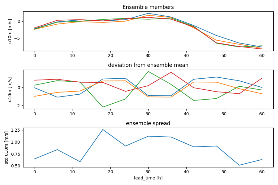
Up first, we can plot a time series of the value of a variable (or statistics of that variable) at a given location (lat/lon coord). In this case lets look at the results predicted over New York.
plt.close("all")
lead_time = np.array(
    (pd.to_datetime(ds.time) - pd.to_datetime(ds.time)[0]).total_seconds() / 3600
)
nyc_lat = 40
nyc_lon = 360 - 74
NYC = ds.sel(lon=nyc_lon, lat=nyc_lat)
fig = plt.figure(figsize=(9, 6))
ax = fig.add_subplot(311)
ax.set_title("Ensemble members")
ax.plot(lead_time, NYC.u10m.T)
ax.set_ylabel("u10m [m/s]")

ax = fig.add_subplot(312)
ax.set_title("deviation from ensemble mean")
ax.plot(lead_time, NYC.t2m.T - NYC.t2m.mean("ensemble"))
ax.set_ylabel("u10m [m/s]")

ax = fig.add_subplot(313)
ax.set_title("ensemble spread")
ax.plot(lead_time, NYC.t2m.std("ensemble"))
ax.set_xlabel("lead_time [h]")
ax.set_ylabel("std u10m [m/s]")
plt.tight_layout()
plt.savefig(f"{output_path}/new_york_zonal_winds.png")
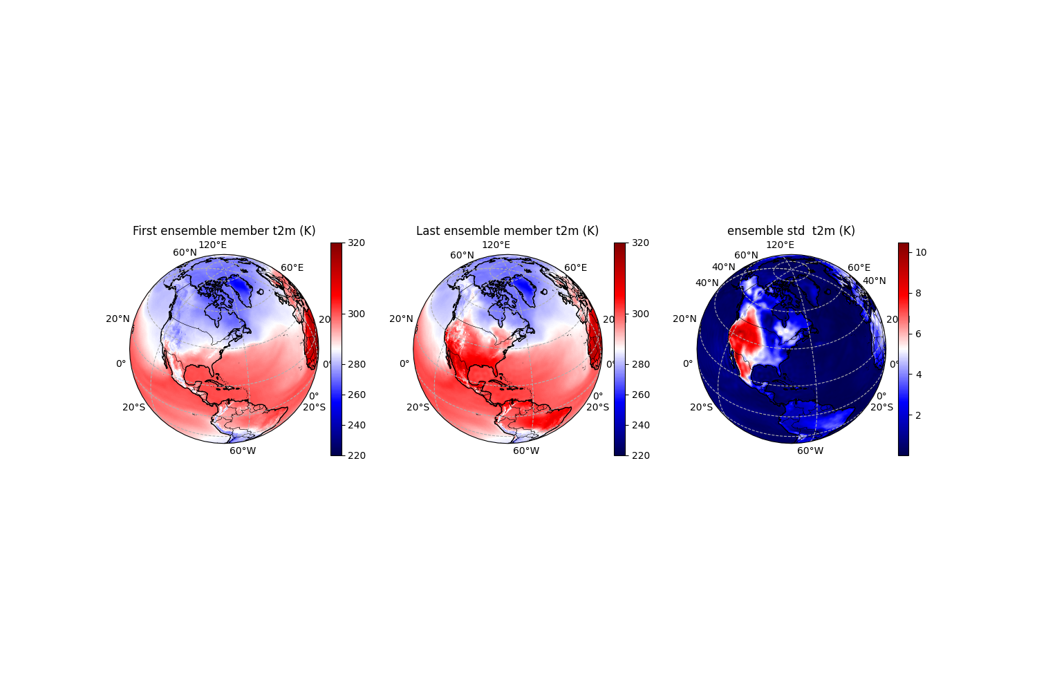
Next, lets plot some fields of surface temperature. Since we have an ensemble of predictions, lets display the first ensemble member, which is deterministic member, and also the last ensemble member and the ensemmble standard deviation. One or both of the perturbed members may look a little noisy, thats because our noise amplitude is maybe too high. Try lowering the amplitude in the config or changing pertibation type to see what happens.
plt.close("all")
fig = plt.figure(figsize=(15, 10))
plt.rcParams["figure.dpi"] = 100
proj = ccrs.NearsidePerspective(central_longitude=nyc_lon, central_latitude=nyc_lat)

data = ds.t2m[0, -1, :, :]
norm = TwoSlopeNorm(vmin=220, vcenter=290, vmax=320)
ax = fig.add_subplot(131, projection=proj)
ax.set_title("First ensemble member t2m (K)")
img = ax.pcolormesh(
    ds.lon, ds.lat, data, transform=ccrs.PlateCarree(), norm=norm, cmap="seismic"
)
ax.coastlines(linewidth=1)
ax.add_feature(countries, edgecolor="black", linewidth=0.25)
plt.colorbar(img, ax=ax, shrink=0.40, norm=mcolors.CenteredNorm(vcenter=0))
gl = ax.gridlines(draw_labels=True, linestyle="--")

data = ds.t2m[-1, -1, :, :]
norm = TwoSlopeNorm(vmin=220, vcenter=290, vmax=320)
ax = fig.add_subplot(132, projection=proj)
plt.rcParams["figure.dpi"] = 100
proj = ccrs.NearsidePerspective(central_longitude=nyc_lon, central_latitude=nyc_lat)
ax.set_title("Last ensemble member t2m (K)")
img = ax.pcolormesh(
    ds.lon, ds.lat, data, transform=ccrs.PlateCarree(), norm=norm, cmap="seismic"
)
ax.coastlines(linewidth=1)
ax.add_feature(countries, edgecolor="black", linewidth=0.25)
plt.colorbar(img, ax=ax, shrink=0.40, norm=mcolors.CenteredNorm(vcenter=0))
gl = ax.gridlines(draw_labels=True, linestyle="--")

ds_ensemble_std = ds.std(dim="ensemble")
data = ds_ensemble_std.t2m[-1, :, :]
# norm = TwoSlopeNorm(vmin=data.min().values, vcenter=5, vmax=data.max().values)
proj = ccrs.NearsidePerspective(central_longitude=nyc_lon, central_latitude=nyc_lat)
ax = fig.add_subplot(133, projection=proj)
ax.set_title("ensemble std  t2m (K)")
img = ax.pcolormesh(ds.lon, ds.lat, data, transform=ccrs.PlateCarree(), cmap="seismic")
ax.coastlines(linewidth=1)
ax.add_feature(countries, edgecolor="black", linewidth=0.25)
plt.colorbar(img, ax=ax, shrink=0.40, norm=mcolors.CenteredNorm(vcenter=0))
gl = ax.gridlines(draw_labels=True, linestyle="--")
plt.savefig(f"{output_path}/gloabl_surface_temp_contour.png")
We can also show a map of the ensemble mean of the 10 meter zonal winds (using some Nvidia style coloring!)
def Nvidia_cmap():
    colors = ["#8946ff", "#ffffff", "#00ff00"]
    cmap = mcolors.LinearSegmentedColormap.from_list("custom_cmap", colors)
    return cmap


plt.close("all")
ds_ensemble_mean = ds.mean(dim="ensemble")
data = ds_ensemble_mean.u10m[-1, :, :]
fig = plt.figure(figsize=(9, 6))
plt.rcParams["figure.dpi"] = 100
proj = ccrs.NearsidePerspective(central_longitude=nyc_lon, central_latitude=nyc_lat)

ax = fig.add_subplot(111, projection=proj)
ax.set_title("ens. mean 10 meter zonal wind [m/s]")
img = ax.pcolormesh(
    ds.lon,
    ds.lat,
    data,
    transform=ccrs.PlateCarree(),
    cmap=Nvidia_cmap(),
    vmin=-20,
    vmax=20,
)
ax.coastlines(linewidth=1)
ax.add_feature(countries, edgecolor="black", linewidth=0.25)
plt.colorbar(img, ax=ax, shrink=0.40, norm=mcolors.CenteredNorm(vcenter=0))
gl = ax.gridlines(draw_labels=True, linestyle="--")
plt.savefig(f"{output_path}/gloabl_mean_zonal_wind_contour.png")
![ens. mean 10 meter zonal wind [m/s]](../_images/sphx_glr_01_ensemble_inference_003.png)
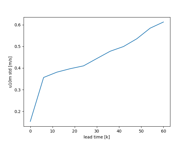
Finally lets compute the latitude-weighted global averages and plot time series of ensemble standard deviation.
def global_average(ds):
    cos_lat = np.cos(np.deg2rad(ds.lat))
    return ds.weighted(cos_lat).mean(["lat", "lon"])


ds_ensemble_std = global_average(ds.std(dim="ensemble"))
plt.close("all")
plt.figure()
plt.plot(lead_time, ds_ensemble_std.u10m)
plt.xlabel("lead time [k]")
plt.ylabel("u10m std [m/s]")
plt.savefig(f"{output_path}/gloabl_std_zonal_surface_wind.png")
And that completes the introductory notebook into running ensemble weather predictions with AI. In the next notebook, we will look at running different models using more Pythonic APIs and plotting geopotential fields.
Total running time of the script: (3 minutes 1.536 seconds)