Scoring Models

The following notebook will demonstrate how to use Earth-2 MIP to perform a scoring workflow to assess the accuracy of AI models using ERA5 reanalysis data as the ground truth. This can then be extended to score custom models placed into the model registry. This tutorial also covers details about using a HDF5 datasource, the expected format this data should be formatted and how to use H5 files for evaluating models over a year’s worth of data.

In summary this notebook will cover the following topics:

• Implementing a basic scoring workflow in Earth-2 MIP

• HDF5 datasource and the expected data format of the H5 files

import datetime
import os

Setting up HDF5 data

The first step of scoring is handling the target data. One could simply use the CDSDatasource to download target data on the fly, but depending on how comprehensive the scoring is, this can prove quite slow. Additionally, many scoring pipelines require on-prem data. Thus, this will demonstrate how to use the HDF5 datasource. The HDF5 data source assumes that the data to be loaded is stored in the general form:

year.h5
    | - field (time, channels, grid)

For DLWP which requires 7 channels with a time-step size of 12 hours, an H5 file will have the following form of data for an entire year:

2017.h5
    | - field (730, 7, 720, 1440)
2016.h5
    | - field (730, 7, 720, 1440)
2015.h5
    | - field (730, 7, 720, 1440)

Note

There is some flexibility with the dimensions of the data in the H5 files. The time dimension may be some factor of 12 (such as 6hr dt or 4hr dt) and the fields may contain additional channels not needed by the model. The data source will select the necessary data for the model. Additionally, the later two dims have some flexibility with regridding.

One option to build these H5 files from scratch is to use the ERA5 mirror scripts provided in Modulus. For the rest of this tutorial, it is assumed that 2017.h5 is present for the full year.

import dotenv

dotenv.load_dotenv()
# can set this with the export ERA5_HDF5=/path/to/root/of/h5/files
h5_folder = os.getenv("ERA5_HDF5")

Loading Models

With the HDF5 datasource loaded the next step is to load our model we wish to score. In this tutorial we will be using the built in FourcastNet model. Take note of the e2mip:// which will direct Earth-2 MIP to load a known model package. FourcastNet is selected here simply because its a 34 channel model which aligns with the H5 files described above.

from modulus.distributed import DistributedManager

from earth2mip import registry
from earth2mip.networks import dlwp

device = DistributedManager().device
package = registry.get_model("e2mip://dlwp")
model = dlwp.load(package, device=device)

HDF5 Datasource

With the H5 files properly formatted, a H5 datasource can now get defined. This requires two items: a root directory location of the H5 files as well as some metadata. Se The metadata is a JSON/dictionary object that helps Earth-2 MIP index the H5 file. Typically, this can be done by placing a data.json file next to the H5 files. See this documentation for more details on how to set up input data correctly.

from earth2mip.initial_conditions import hdf5

datasource = hdf5.DataSource.from_path(
    root=h5_folder, channel_names=model.channel_names
)

# Test to see if our datasource is working
time = datetime.datetime(2017, 5, 1, 18)
out = datasource[time]
print(out.shape)

(7, 721, 1440)

Running Scoring

With the datasource and model loaded, scoring can now be performed. To score this we will run 10 day forecasts over the span of the entire year at 30 day intervals. For research, one would typically want this to be much more comprehensive so feel free to customize for you’re use case.

The score_deterministic API provides a simple way to calculate RMSE and ACC scores. ACC scores require climatology which is beyond the scope of this example, thus zero values will be provided and only the RMSE will be of concern. This function will save the results of every inference run into a CSV file which can then be pose process using some of the utility functions Earth-2 MIP provides.

from earth2mip.inference_medium_range import save_scores, time_average_metrics

# Use 12 initializations.
time = datetime.datetime(2017, 1, 2, 0)
initial_times = [
    time + datetime.timedelta(days=30 * i, hours=6 * i) for i in range(12)
]  # modify here to change the initializations

# Output directoy
output_dir = "outputs/03_model_scoring"
if not os.path.exists(output_dir):
    os.makedirs(output_dir, exist_ok=True)
    output = save_scores(
        model,
        n=28,  # 6 hour timesteps (28*6/24 = 7-day forecast)
        initial_times=initial_times,
        data_source=datasource,
        time_mean=datasource.time_means,
        output_directory=output_dir,
    )

Post Processing

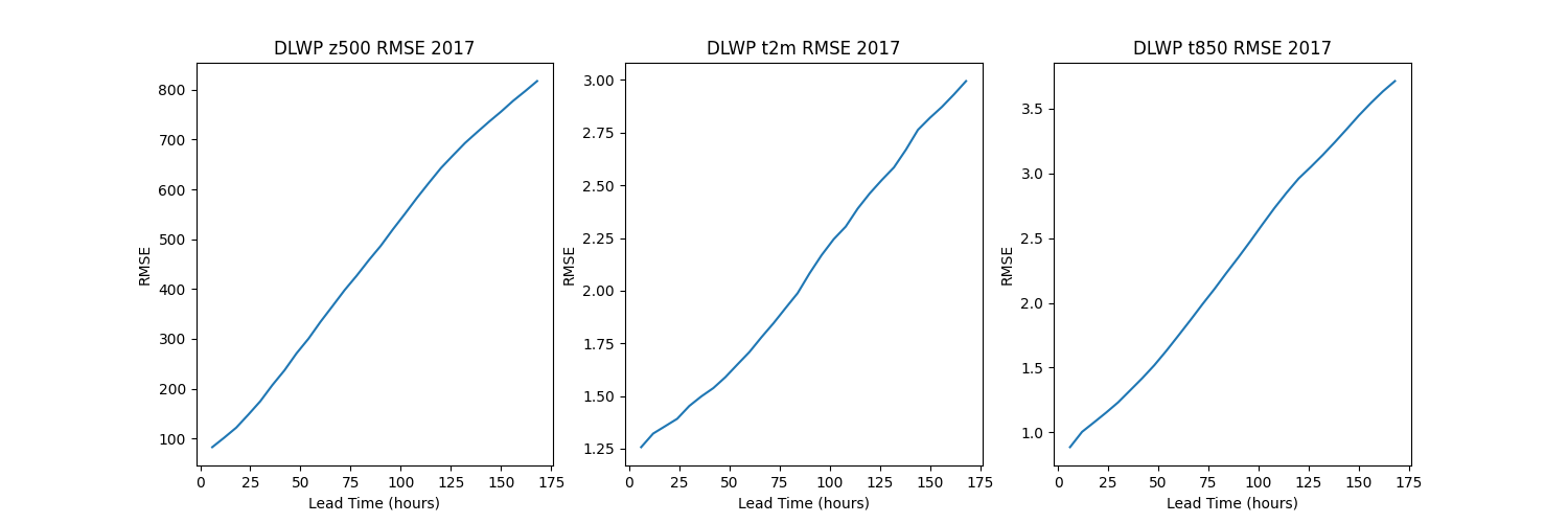
The last step is any post processing / IO that is desired. Typically its recommended to save the output dataset to a netCDF file for further processing. Lets plot the RMSE of the z500 (geopotential at pressure level 500) field.

import matplotlib.pyplot as plt
import pandas as pd

from earth2mip.forecast_metrics_io import read_metrics

series = read_metrics(output_dir)
dataset = time_average_metrics(series)

plt.close("all")
fig, axs = plt.subplots(1, 3, figsize=(15, 5))
channels = ["z500", "t2m", "t850"]
t = dataset.lead_time / pd.Timedelta("1 h")
for i, channel in enumerate(channels):
    y = dataset.rmse.sel(channel=channel)
    axs[i].plot(t[1:], y[1:])  # Ignore first output as that's just initial condition.
    axs[i].set_xlabel("Lead Time (hours)")
    axs[i].set_ylabel("RMSE")
    axs[i].set_title(f"DLWP {channel} RMSE 2017")

plt.savefig(f"{output_dir}/dwlp_rmse.png")

This completes this introductory notebook on basic scoring of models in Earth-2 MIP, which is founational for comparing the performance of different models.