Diagnostic Models for Precipitation

The following notebook will demonstrate how to use diagnostic models inside of Earth-2 MIP for transforming outputs of global weather models into different quantities of interest. More information on diagnostics can be found in the user guide.

In summary this notebook will cover the following topics:

• Loading a built in diagnostic model for predicting total precipitation

• Combining the diagnostic model with a prognostic model using the DiangosticLooper

import datetime
import os
import dotenv

dotenv.load_dotenv()

True

Loading Diagnostic Models

Loading diagnostic models is similar to prognostic models, but presently use a slightly different API. In this example we will using the built in AFNO FourCast Net to serve as the underlying prognostic model that will drive the time-ingration. The PrecipitationAFNO model will then be used to “post-process” the outputs of this model to predict precipitation. The key API to load a diagnostic model is the load_diagnostic(package) function which takes a model package in. If you’re interested in using the built in model package (i.e. checkpoint), then the load_package() function can do this for you.

from modulus.distributed.manager import DistributedManager
from earth2mip.networks import get_model
from earth2mip.diagnostic import PrecipitationAFNO

device = DistributedManager().device

print("Loading FCN model")
model = get_model("e2mip://fcn", device=device)

print("Loading precipitation model")
package = PrecipitationAFNO.load_package()
diagnostic = PrecipitationAFNO.load_diagnostic(package)

Loading FCN model
Loading precipitation model

The next step is to wrap the prognostic model with the Diagnostic Time loop. Essentially this adds the execution of the diagnostic model on top of the forecast model iterator. This will add the total preciptation field (tp) to the output data which can the be further processed.

from earth2mip.diagnostic import DiagnosticTimeLoop

model_diagnostic = DiagnosticTimeLoop(diagnostics=[diagnostic], model=model)

Running Inference

With the diagnostic time loop created the final steps are to create the data source and run inference. For this example we will use the CDS data source again. Its assumed your CDS API key is already set up. Reference the first example for additional information. We will use the basic inference workflow which returns a Xarray dataset we will save to netCDF.

from earth2mip.inference_ensemble import run_basic_inference
from earth2mip.initial_conditions import cds

print("Constructing initializer data source")
data_source = cds.DataSource(model.in_channel_names)
time = datetime.datetime(2018, 4, 4)

print("Running inference")
output_dir = "outputs/04_diagnostic_precip"
os.makedirs(output_dir, exist_ok=True)
ds = run_basic_inference(
    model_diagnostic,
    n=20,
    data_source=data_source,
    time=time,
)
ds.to_netcdf(os.path.join(output_dir, "precipitation_afno.nc"))
print(ds)

Constructing initializer data source
Running inference
<xarray.DataArray (time: 21, history: 1, channel: 27, lat: 720, lon: 1440)>
array([[[[[-2.11471558e-01, -2.11471558e-01, -2.11471558e-01, ...,
           -2.11471558e-01, -2.11471558e-01, -2.11471558e-01],
          [-3.07084632e+00, -3.06889343e+00, -3.06596375e+00, ...,
           -3.07865906e+00, -3.07572937e+00, -3.07377601e+00],
          [-2.84233093e+00, -2.83549500e+00, -2.83061218e+00, ...,
           -2.85795593e+00, -2.85307312e+00, -2.84819031e+00],
          ...,
          [-5.65287781e+00, -5.62846375e+00, -5.60502625e+00, ...,
           -5.70756531e+00, -5.68901062e+00, -5.67143297e+00],
          [-4.96537781e+00, -4.94975281e+00, -4.92436218e+00, ...,
           -5.02104187e+00, -4.99662781e+00, -4.97807312e+00],
          [-3.68022156e+00, -3.66361976e+00, -3.64799523e+00, ...,
           -3.71830750e+00, -3.70561218e+00, -3.69291711e+00]],

         [[-3.34625393e-02, -3.34625393e-02, -3.34625393e-02, ...,
           -3.34625393e-02, -3.34625393e-02, -3.34625393e-02],
          [ 4.14779663e-01,  4.18685913e-01,  4.21615601e-01, ...,
            4.01107788e-01,  4.05990601e-01,  4.09896851e-01],
          [ 9.58724976e-01,  9.62631226e-01,  9.68490601e-01, ...,
            9.35287476e-01,  9.44076598e-01,  9.51889098e-01],
...
            2.08597885e+02,  2.08562744e+02,  2.08502136e+02],
          [ 2.09902100e+02,  2.09973709e+02,  2.09911636e+02, ...,
            2.08666016e+02,  2.08584030e+02,  2.08495407e+02],
          [ 2.09857300e+02,  2.09878571e+02,  2.09833130e+02, ...,
            2.08613449e+02,  2.08585724e+02,  2.08611252e+02]],

         [[ 5.76145576e-05,  6.56552511e-05,  6.22156876e-05, ...,
            5.97032849e-05,  5.60570406e-05,  6.52155722e-05],
          [ 6.52452145e-05,  6.69267029e-05,  6.32969095e-05, ...,
            5.56269479e-05,  5.41082591e-05,  6.48130372e-05],
          [ 6.78307624e-05,  6.97310606e-05,  7.20787430e-05, ...,
            6.11619107e-05,  5.68764190e-05,  6.89467197e-05],
          ...,
          [ 4.73785758e-06,  3.20812342e-06,  3.82903818e-06, ...,
            7.07706795e-06,  6.76194668e-06,  4.07153220e-06],
          [ 6.52008976e-06,  4.05368928e-06,  4.89662170e-06, ...,
            7.27669340e-06,  9.10134622e-06,  7.08135121e-06],
          [ 1.25541401e-05,  9.00194118e-06,  8.55812050e-06, ...,
            1.23706168e-05,  1.38230034e-05,  1.21808262e-05]]]]],
      dtype=float32)
Coordinates:
  * lat      (lat) float64 90.0 89.75 89.5 89.25 ... -89.0 -89.25 -89.5 -89.75
  * lon      (lon) float64 0.0 0.25 0.5 0.75 1.0 ... 359.0 359.2 359.5 359.8
  * channel  (channel) <U5 'u10m' 'v10m' 't2m' 'sp' ... 'z250' 't250' 'tp'
  * time     (time) datetime64[ns] 2018-04-04 2018-04-04T06:00:00 ... 2018-04-09
Dimensions without coordinates: history

Post Processing

With inference complete we can do some post processing on our predictions. Lets first visualize the total precipitation and total column water vapor for a few days.

import cartopy
import cartopy.crs as ccrs
import matplotlib.pyplot as plt
import numpy as np
import pandas as pd
import xarray as xr


plt.close("all")
# Open dataset from saved NetCDFs
ds = xr.open_dataarray(os.path.join(output_dir, "precipitation_afno.nc"))

ndays = 3
proj = ccrs.Robinson()
fig, ax = plt.subplots(
    2,
    ndays,
    figsize=(15, 5),
    subplot_kw={"projection": proj},
    gridspec_kw={"wspace": 0.05, "hspace": 0.007},
)

for day in range(ndays):
    i = 4 * day  # 6-hour timesteps
    tp = ds[i, 0].sel(channel="tp")
    img = ax[0, day].pcolormesh(
        tp.lon,
        tp.lat,
        tp.values,
        transform=ccrs.PlateCarree(),
        cmap="cividis",
        vmin=0,
        vmax=0.05,
    )
    ax[0, day].set_title(pd.to_datetime(ds.coords["time"])[i])
    ax[0, day].coastlines(color="k")
    plt.colorbar(img, ax=ax[0, day], shrink=0.40)

    tcwv = ds[i, 0].sel(channel="tcwv")
    img = ax[1, day].pcolormesh(
        tcwv.lon,
        tcwv.lat,
        tcwv.values,
        transform=ccrs.PlateCarree(),
        cmap="gist_ncar",
        vmin=0,
        vmax=75,
    )
    ax[1, day].coastlines(resolution="auto", color="k")
    plt.colorbar(img, ax=ax[1, day], shrink=0.40)

ax[0, 0].text(
    -0.07,
    0.55,
    "Total Precipitation (m)",
    va="bottom",
    ha="center",
    rotation="vertical",
    rotation_mode="anchor",
    transform=ax[0, 0].transAxes,
)

ax[1, 0].text(
    -0.07,
    0.55,
    "Total Column\nWater Vapor (kg m-2)",
    va="bottom",
    ha="center",
    rotation="vertical",
    rotation_mode="anchor",
    transform=ax[1, 0].transAxes,
)

plt.savefig(f"{output_dir}/diagnostic_tp_tcwv.png")

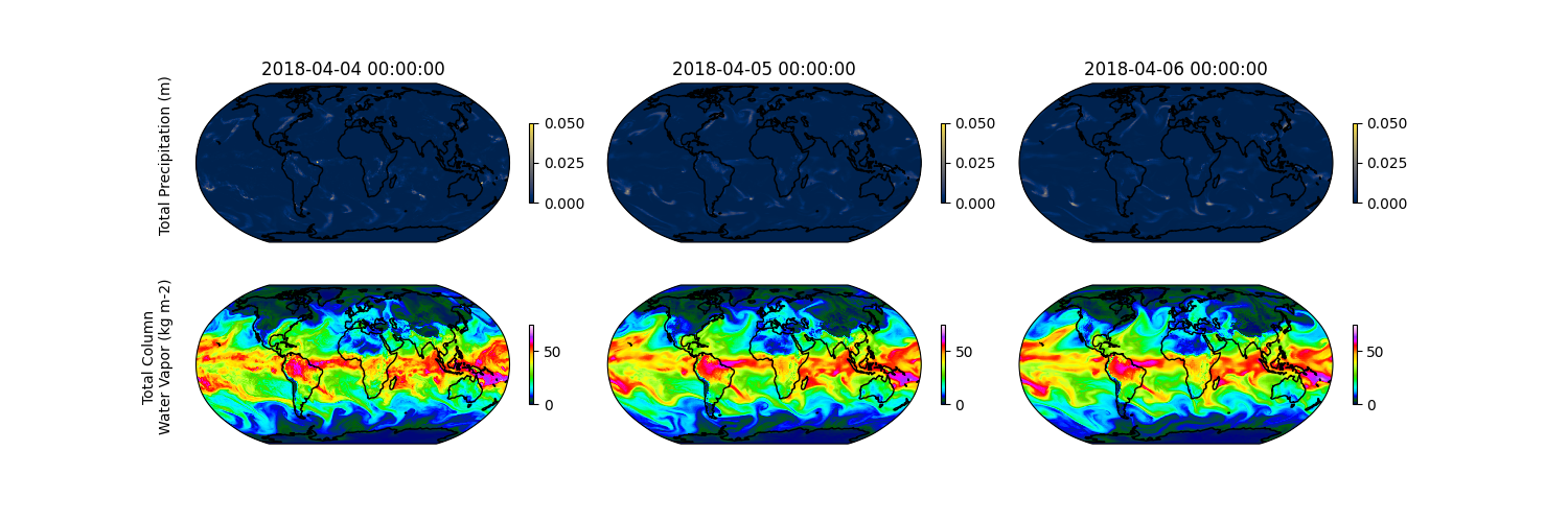
This partiulcar date was selected for inference due to an atmopsheric river occuring over the west coast of the United States. Lets plot the total precipitation that occured over San Francisco.

plt.close("all")
# Open dataset from saved NetCDFs
ds = xr.open_dataarray(os.path.join(output_dir, "precipitation_afno.nc"))

tp_sf = ds.sel(channel="tp", lat=37.75, lon=57.5)  # Lon is [0, 360]

plt.plot(pd.to_datetime(tp_sf.coords["time"]), tp_sf.values)
plt.title("SF (lat: 37.75N lon: 122.5W)")
plt.ylabel("Total Precipitation (m)")
plt.savefig(f"{output_dir}/sf_tp.png")

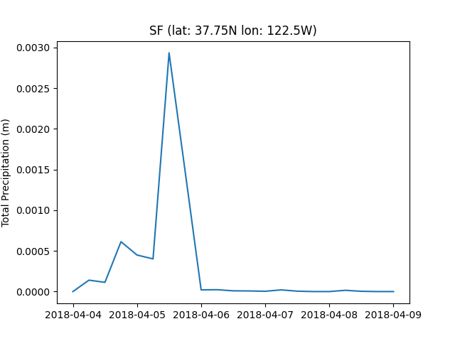
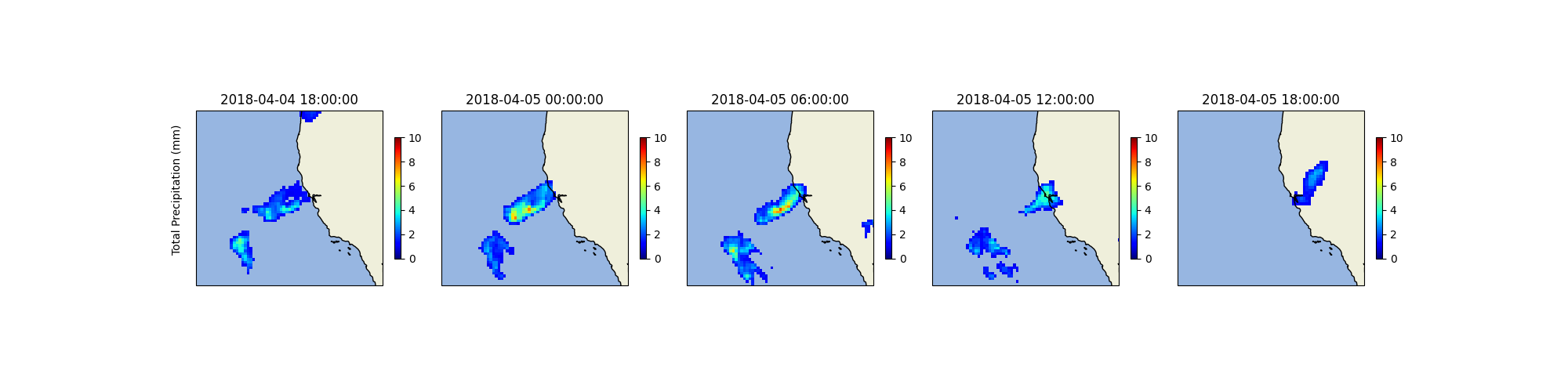
The land fall of the atmosphric river is very clear here, lets have a look at the regional contour of the bay area to better understand the structure of this event.

plt.close("all")
# Open dataset from saved NetCDFs
ds = xr.open_dataarray(os.path.join(output_dir, "precipitation_afno.nc"))
nsteps = 5
proj = ccrs.AlbersEqualArea(central_latitude=37.75, central_longitude=-122.5)
fig, ax = plt.subplots(
    1,
    nsteps,
    figsize=(20, 5),
    subplot_kw={"projection": proj},
    gridspec_kw={"wspace": 0.05, "hspace": 0.007},
)

for step in range(nsteps):
    i = step + 3
    tp = ds[i, 0].sel(channel="tp")

    ax[step].add_feature(cartopy.feature.OCEAN, zorder=0)
    ax[step].add_feature(cartopy.feature.LAND, zorder=0)
    masked_data = np.ma.masked_where(tp.values < 0.001, tp.values)
    img = ax[step].imshow(
        1000 * masked_data,
        transform=ccrs.PlateCarree(),
        cmap="jet",
        vmin=0,
        vmax=10,
    )
    ax[step].set_title(pd.to_datetime(ds.coords["time"])[i])
    ax[step].coastlines(color="k")
    ax[step].set_extent([-115, -135, 30, 45], ccrs.PlateCarree())
    plt.colorbar(img, ax=ax[step], shrink=0.40)


ax[0].text(
    -0.07,
    0.55,
    "Total Precipitation (mm)",
    va="bottom",
    ha="center",
    rotation="vertical",
    rotation_mode="anchor",
    transform=ax[0].transAxes,
)

plt.savefig(f"{output_dir}/diagnostic_bay_area_tp.png")

This completes the introductory notebook on running diagnostic models. Diangostic models are signifcantly more cheap to train and more flexible for difference usecases. In later examples, we will explore using these models of various other tasks.