Dynamics Benchmarks#
This page presents benchmark results for molecular dynamics (MD) integrators and geometry optimization methods using the nvalchemiops GPU-accelerated implementations. Results show scaling behavior for both single-system and batched simulations across different system sizes using Lennard-Jones argon systems.
Warning
These results are intended to be indicative only: your actual performance may vary depending on the atomic system topology, software and hardware configuration and we encourage users to benchmark on their own systems of interest.
How to Read These Charts#
Time Scaling : Average time per MD/optimization step (ms) vs. system size. Lower is better. For batched runs, this is the time to process all systems in the batch.
Throughput : Atom-steps processed per second. Higher is better. For batched systems, this represents the total number of atoms across all systems in the batch multiplied by the number of steps per second.
Ensemble : MD ensemble type - NVE (constant energy), NVT (constant temperature), NPT (constant pressure-temperature), or NPH (constant pressure-enthalpy).
Batch Size : Number of independent systems processed simultaneously. Batch size of 1 represents single-system mode.
Molecular Dynamics (MD)#
GPU-accelerated MD integrators using NVIDIA Warp kernels with optimized neighbor lists. Supports various ensembles including microcanonical (NVE), canonical (NVT), and isobaric-isothermal (NPT).
Single-System MD#
Performance for single molecular dynamics systems showing how throughput scales with system size.
Time Scaling#
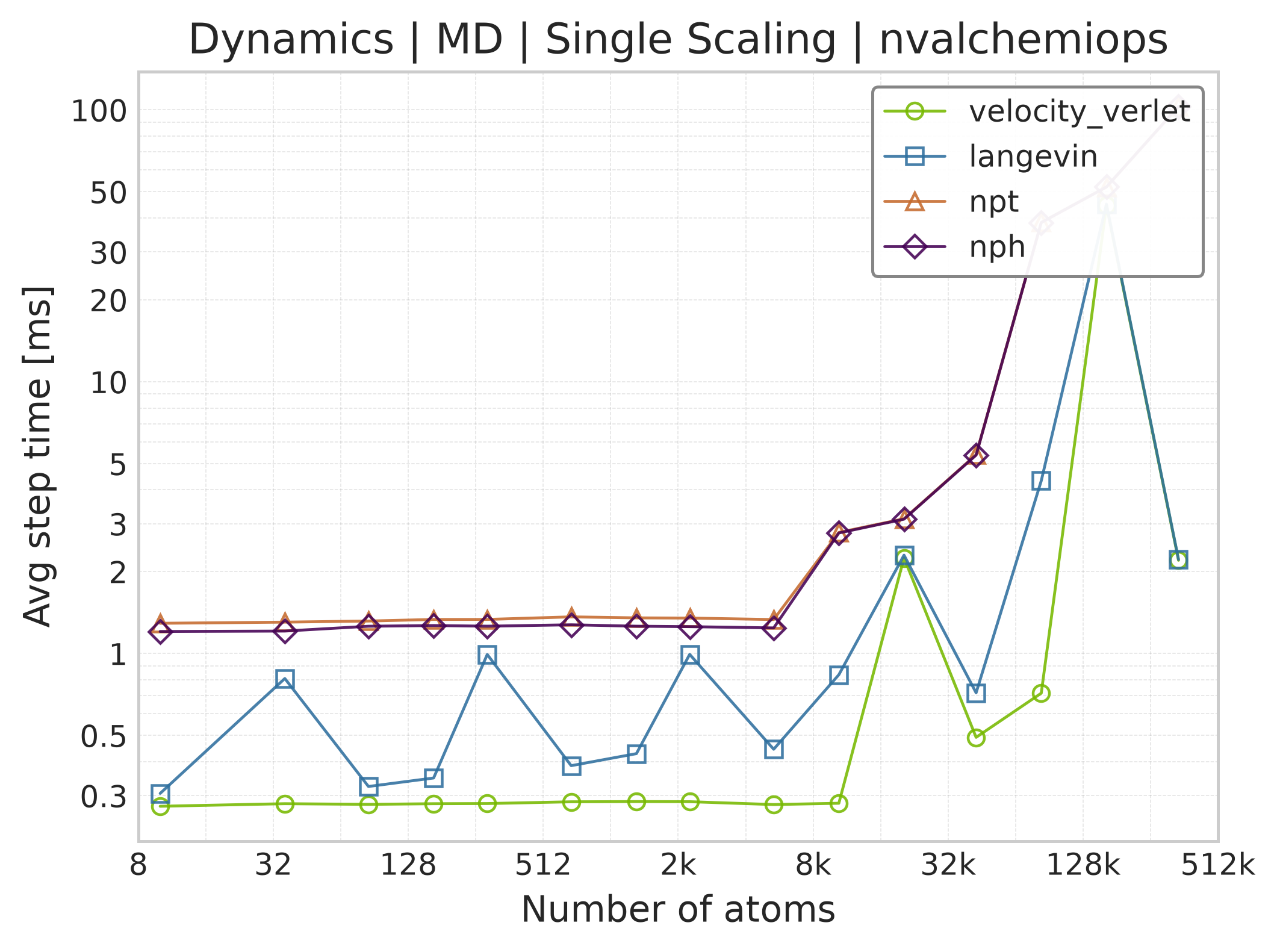
Average step time vs. system size for single-system MD integrators.#
Throughput#
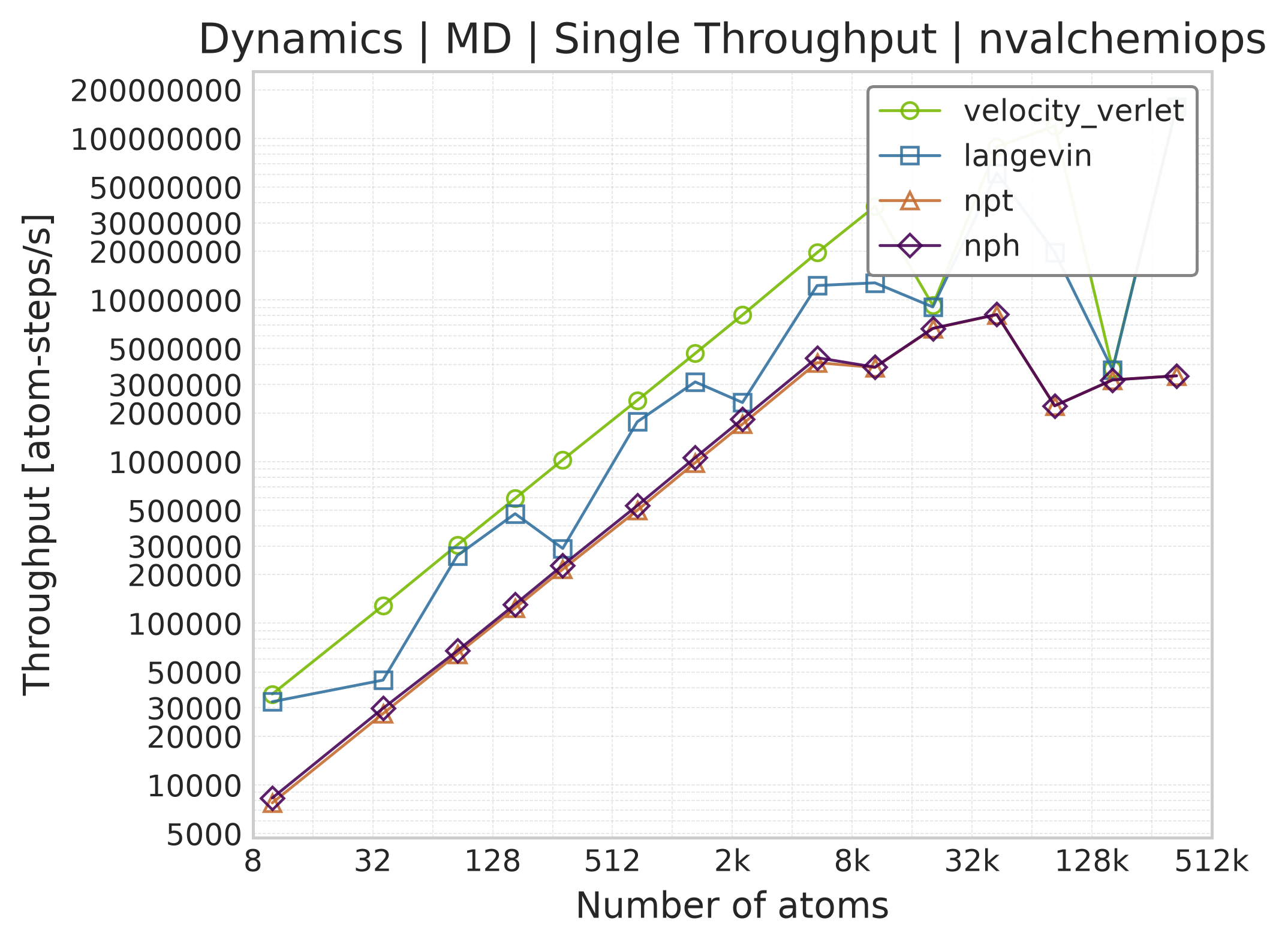
Throughput (atom-steps/s) for single-system MD integrators.#
Available Integrators#
Velocity Verlet (NVE) : Symplectic integrator that conserves total energy. Excellent stability for constant energy simulations. Standard choice for microcanonical ensemble.
Langevin (NVT) : Stochastic dynamics using the BAOAB splitting scheme for accurate temperature control. Maintains canonical ensemble through friction and random forces.
Nose-Hoover Chain (NVT) : Deterministic thermostat using extended system variables. Provides rigorous canonical sampling without stochastic forces.
NPT Integrator : Isobaric-isothermal ensemble allowing cell fluctuations to maintain constant pressure and temperature. Uses Nose-Hoover chains for temperature control and barostat for pressure control.
NPH Integrator : Isobaric-enthalpic ensemble with constant pressure. Similar to NPT but without temperature control.
Geometry Optimization#
GPU-accelerated FIRE and FIRE2 (Fast Inertial Relaxation Engine) optimizers for efficient energy minimization. Both adapt timestep and velocity-force mixing for robust convergence on diverse energy landscapes. FIRE2 (Guénolé et al., 2020) introduces a deferred half-step and modified velocity mixing for improved convergence behavior. A quasi-Newton L-BFGS optimizer is also available; the sections below compare it against FIRE2 on evaluation count and per-step cost.
Single-System Optimization#
Performance for single-system geometry optimization showing convergence speed and computational efficiency.
Time Scaling#
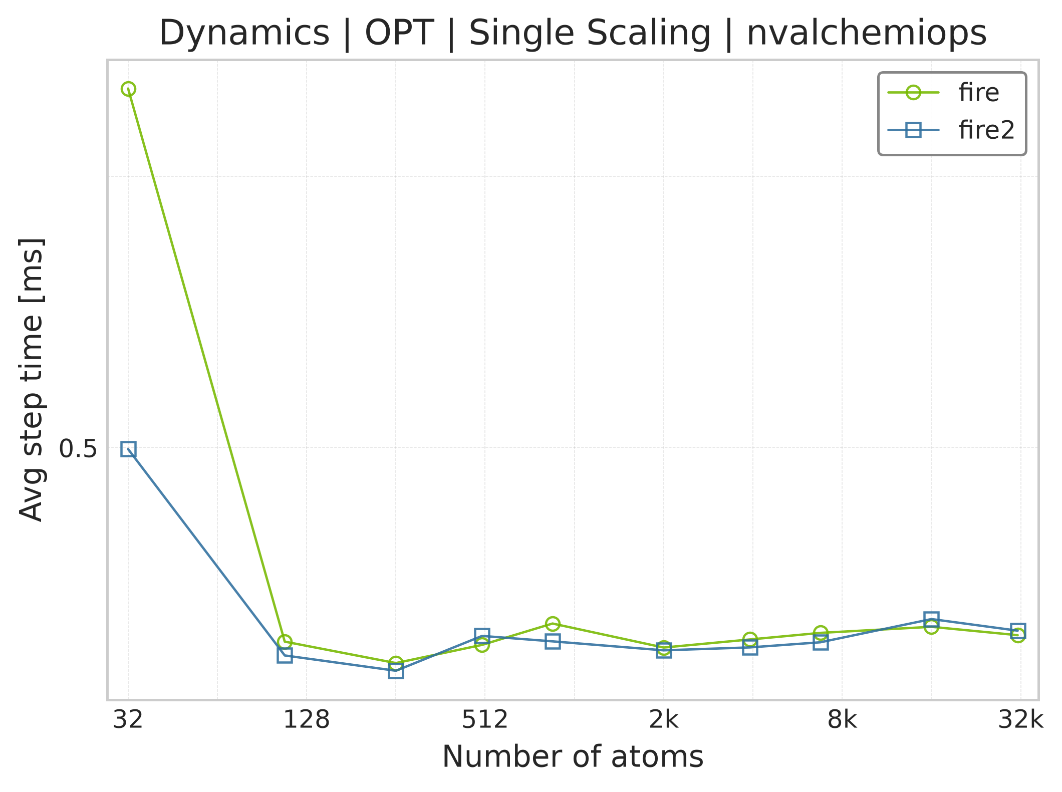
Average step time vs. system size for FIRE optimizer.#
Throughput#
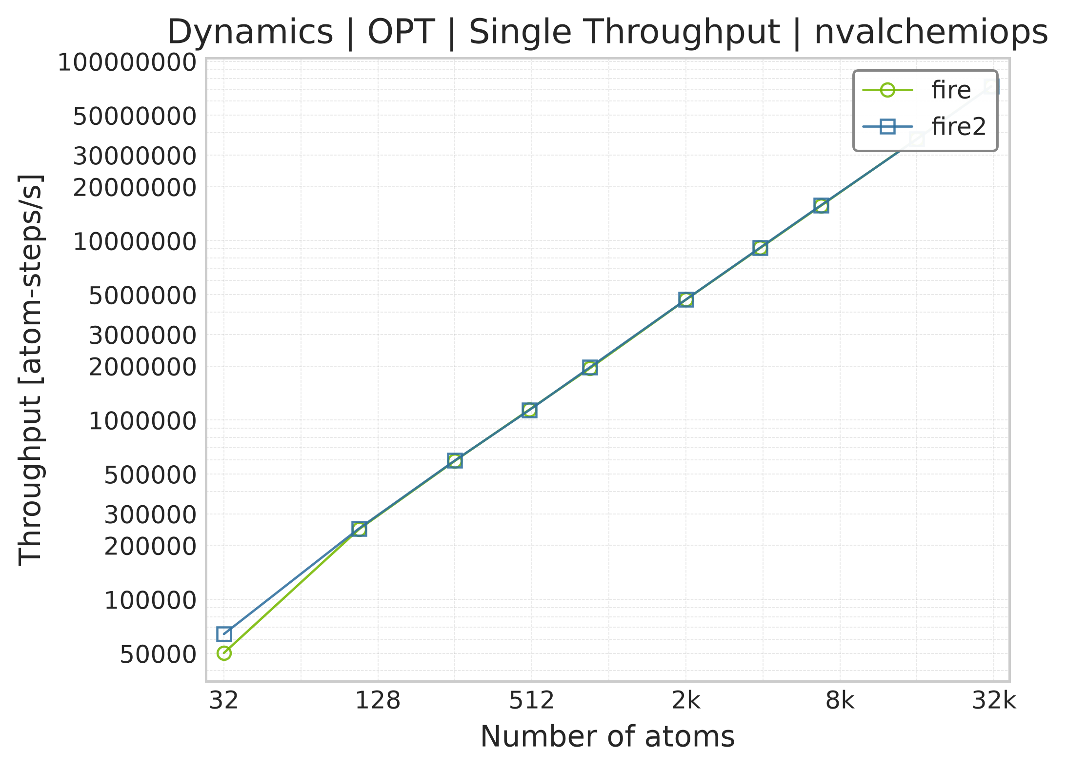
Throughput (atom-steps/s) during geometry optimization.#
Batched Optimization#
Performance for batched optimization showing how multiple structures can be relaxed simultaneously for efficient saddle point searches, transition state finding, or structural screening.
Time Scaling#
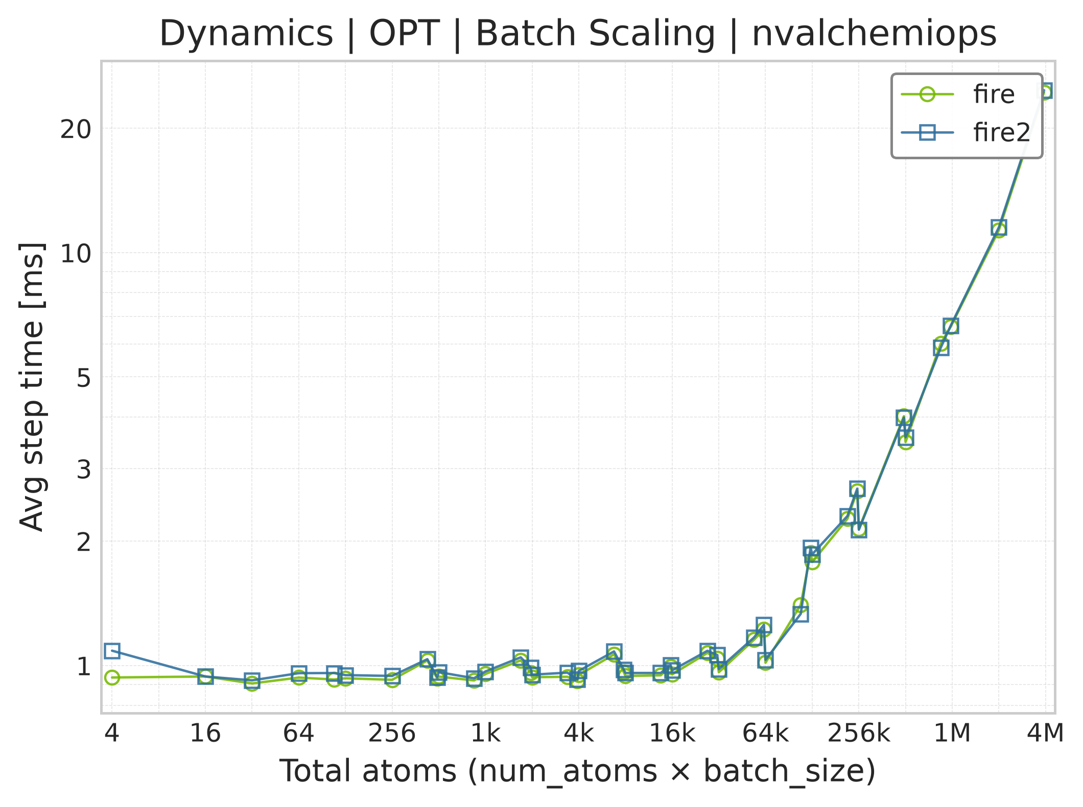
Average step time for batched FIRE optimization.#
Throughput#
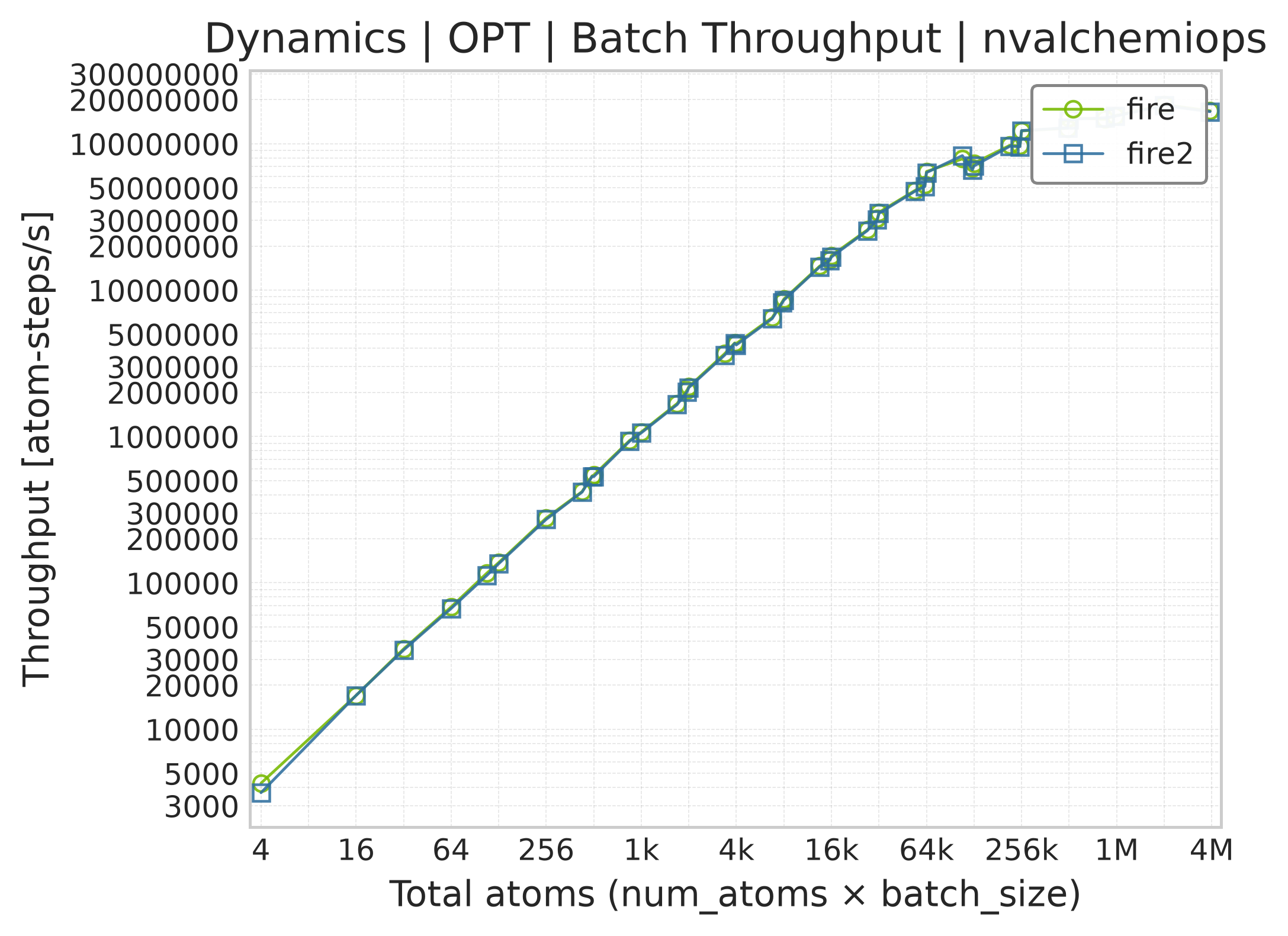
Total throughput (atom-steps/s) for batched optimization.#
L-BFGS vs FIRE2: Algorithm Design and Benchmark Evidence#
Energy minimization methods balance two competing costs: the number of force evaluations to reach convergence, and the computational overhead of the optimizer per step.
The algorithms.
FIRE2 (Fast Inertial Relaxation Engine 2) treats optimization as damped molecular dynamics. The algorithm adjusts velocities along the force direction and dynamically adapts the integration timestep:
Adaptive timestep: After
delaystep(default 60) consecutive downhill steps (\(P = \mathbf{F} \cdot \mathbf{v} > 0\)), the timestep grows by factordtgrow(default 1.05) up totmax(default 0.08). On an uphill step it shrinks bydtshrink(default 0.75), bounded below bytmin(default 0.005).Velocity mixing: Mixes velocity with the normalized force direction: \(\mathbf{v} \leftarrow (1-\alpha)\mathbf{v} + \alpha |\mathbf{v}| \hat{\mathbf{F}}\). Downhill, the mixing parameter decays by
alphashrink(default 0.985); uphill, it resets toalpha0(default 0.09).Maximum displacement: Limits each system’s step to
maxstep(default 0.1) for stability.Caller-owned stopping:
fire2_stephas no tolerance and no terminal status. The caller checks convergence, for example by the largest per-atom force magnitude, and decides when to stop.
L-BFGS (Limited-memory Broyden-Fletcher-Goldfarb-Shanno) is a quasi-Newton
optimization method. It approximates the inverse Hessian operator from a rolling
history of \(m\) past displacement and force-difference vectors (typically \(m \in [3,
7]\)). At each step, L-BFGS calculates a descent direction with a two-loop recursion
and takes a step bounded by a maxstep trust region (default \(0.2\,\text{Å}\)).
State and step cost.
Both optimizers evaluate atomic forces once per step. The L-BFGS implementation bounds steps with a trust region rather than a line search, avoiding extra energy evaluations.
The required memory and computation per step differ:
State memory: FIRE2 stores atomic positions, velocities, and scalar parameters (\(\Delta t, \alpha\)). L-BFGS stores positions, forces, and \(m\) history pairs of displacement and force differences. For \(P\) degrees of freedom, L-BFGS history requires \((2m + \mathcal{O}(1))\) vectors in memory.
Compute per step: FIRE2 requires only vector additions and scalar reductions. L-BFGS executes a two-loop recursion over history (\((2m + \mathcal{O}(1))\) vector passes), which increases GPU overhead per step.
Evaluations to convergence.
The table below compares force evaluations to reach convergence (\(\max_i \lVert \mathbf{F}_i \rVert < 10^{-4}\,\text{eV}/\text{Å}\)). The test uses argon clusters of 13, 32, and 55 atoms across five initial geometries per size. FIRE2 timesteps were swept over eight settings to establish the baseline.
Metric |
float32 |
float64 |
|---|---|---|
Geometric mean of L-BFGS/FIRE2 evaluation counts |
0.59 |
0.57 |
Worst ratio in this sample |
0.94 |
1.08 |
Cases where both converged |
15 / 15 |
15 / 15 |
In this synthetic sample, L-BFGS converged in roughly 40% fewer force evaluations than FIRE2 on average.
Per-step optimizer cost.
The table below compares optimizer execution time per step for a single system using harmonic interactions. The measurement isolates optimizer kernel time from force evaluation time.
Atoms |
Precision |
Eager (ms) |
CUDA graph (ms) |
FIRE2 (ms) |
vs FIRE2 |
|---|---|---|---|---|---|
10,000 |
float32 |
0.46 |
0.15 |
0.052 |
8.8x |
10,000 |
float64 |
0.44 |
0.18 |
0.056 |
7.9x |
100,000 |
float32 |
1.06 |
1.06 |
0.130 |
8.2x |
100,000 |
float64 |
1.10 |
1.11 |
0.119 |
9.3x |
1,000,000 |
float32 |
3.52 |
3.53 |
0.289 |
12.2x |
1,000,000 |
float64 |
5.00 |
5.00 |
0.353 |
14.2x |
Across these test sizes, L-BFGS per-step time is \(7.9\times\) to \(14.2\times\) higher than FIRE2. CUDA graph capture reduces launch overhead for smaller systems.
Break-even trade-off.
The faster optimizer for a given workflow depends on the cost of the force calculation:
When force evaluation takes more than a few milliseconds per step (typical for neural network potentials or DFT), evaluation count dominates total runtime, favoring the optimizer with fewer evaluations in this benchmark.
When force evaluation is fast (typical for empirical pair potentials), optimizer overhead dominates total runtime, favoring the optimizer with the cheaper step.
Because these results come from a synthetic benchmark on small Lennard-Jones clusters, benchmark both optimizers on your target structures and potentials before choosing.
For complete optimization workflows, see the FIRE2 Geometry Optimization (LJ Cluster) and L-BFGS Geometry Optimization (LJ Cluster) gallery examples.
Hardware Information#
GPU: NVIDIA H100 80GB HBM3
Benchmark Configuration#
The checked-in dynamics CSVs carry the measured atom counts, step counts,
timestep, and warmup count for each row. The single-system MD snapshot uses
1,000 steps, a 0.001 fs timestep, and 100 untimed warmup steps. Current runner
defaults, including the 94.4 K single-system thermostat settings and all size
grids, live in benchmarks/dynamics/benchmark_config.yaml.
Dynamics results use their own historical schema and are not part of the reportable NL/D3/electrostatics 18-file snapshot. When reproducing a plotted dynamics point, treat the committed CSV row as the record of that measurement and the YAML as the configuration for a new run.
Running Your Own Benchmarks#
To reproduce these benchmarks or test on your own hardware:
Single-System MD#
cd benchmarks/dynamics
python benchmark_md_single.py --config benchmark_config.yaml
Batched MD#
python benchmark_md_batch.py --config benchmark_config.yaml
Single-System Optimization#
python benchmark_opt_single.py --config benchmark_config.yaml
Batched Optimization#
python benchmark_opt_batch.py --config benchmark_config.yaml
FIRE1 vs FIRE2 Comparison#
Full optimization runs comparing FIRE1 and FIRE2 convergence and wall-clock time on fixed-cell and variable-cell LJ systems:
python benchmark_fire_compare.py --config benchmark_config.yaml --output-dir ./benchmark_results
FIRE2 Kernel Performance#
Raw per-step GPU kernel timing using CUDA events, sweeping total atoms and batch sizes across float32 and float64:
python benchmark_fire2.py --config benchmark_config.yaml --output-dir ./benchmark_results
L-BFGS vs FIRE2#
Energy/force evaluations to convergence, which is the cost that dominates relaxation driven by a machine-learned potential, plus per-step cost gates:
python benchmark_lbfgs.py --config benchmark_config.yaml --output-dir ./benchmark_results
python benchmark_lbfgs.py --gates
FIRE2 is swept over the grid in the config’s lbfgs.fire2_sweep block and its
best converged result is what L-BFGS is compared against, so the baseline is not
handicapped by an untuned timestep.
Configuration File#
Edit benchmarks/dynamics/benchmark_config.yaml to select current size grids,
integrators, optimizers, and timing parameters. Keeping the executable YAML as
the single configuration source avoids stale copies in the documentation.
Output#
Results are saved as CSV files in docs/benchmarks/benchmark_results/:
dynamics_md_single_nvalchemiops_<gpu_sku>.csvdynamics_opt_single_nvalchemiops_<gpu_sku>.csvdynamics_opt_batch_nvalchemiops_<gpu_sku>.csvfire_compare_<gpu_sku>.csvfire2_kernel_benchmark_<gpu_sku>.csv
Generate plots with:
cd docs/benchmarks
python generate_plots.py