Electrostatics Benchmarks

This page presents benchmark results for electrostatic interaction methods including Ewald summation, Particle Mesh Ewald (PME), and Damped Shifted Force (DSF) across different GPU hardware. Results show the scaling behavior with increasing system size for both single-system and batched computations.

Warning

These results are intended to be indicative only: your actual performance may vary depending on the atomic system topology, software and hardware configuration and we encourage users to benchmark on their own systems of interest.

How to Read These Charts

Time Scaling : Median execution time (ms) vs. system size. Lower is better. Timings include both real-space and reciprocal-space contributions when running “full” mode.

Throughput : Atoms processed per millisecond. Higher is better. This indicates the scaling point where the GPU saturates.

Memory : Peak GPU memory usage (MB) vs. system size. This is particularly useful for estimating/gauging memory requirements for your system.

Ewald Summation

The Ewald summation method splits the Coulomb interaction into real-space and reciprocal-space components. This is the traditional \(O(N^{3/2})\) to \(O(N^2)\) method depending on parameter choices.

Backend Comparison

Simple comparison of single (non-batched) system computations between backends, where we scale up the size of the supercell.

Time Scaling

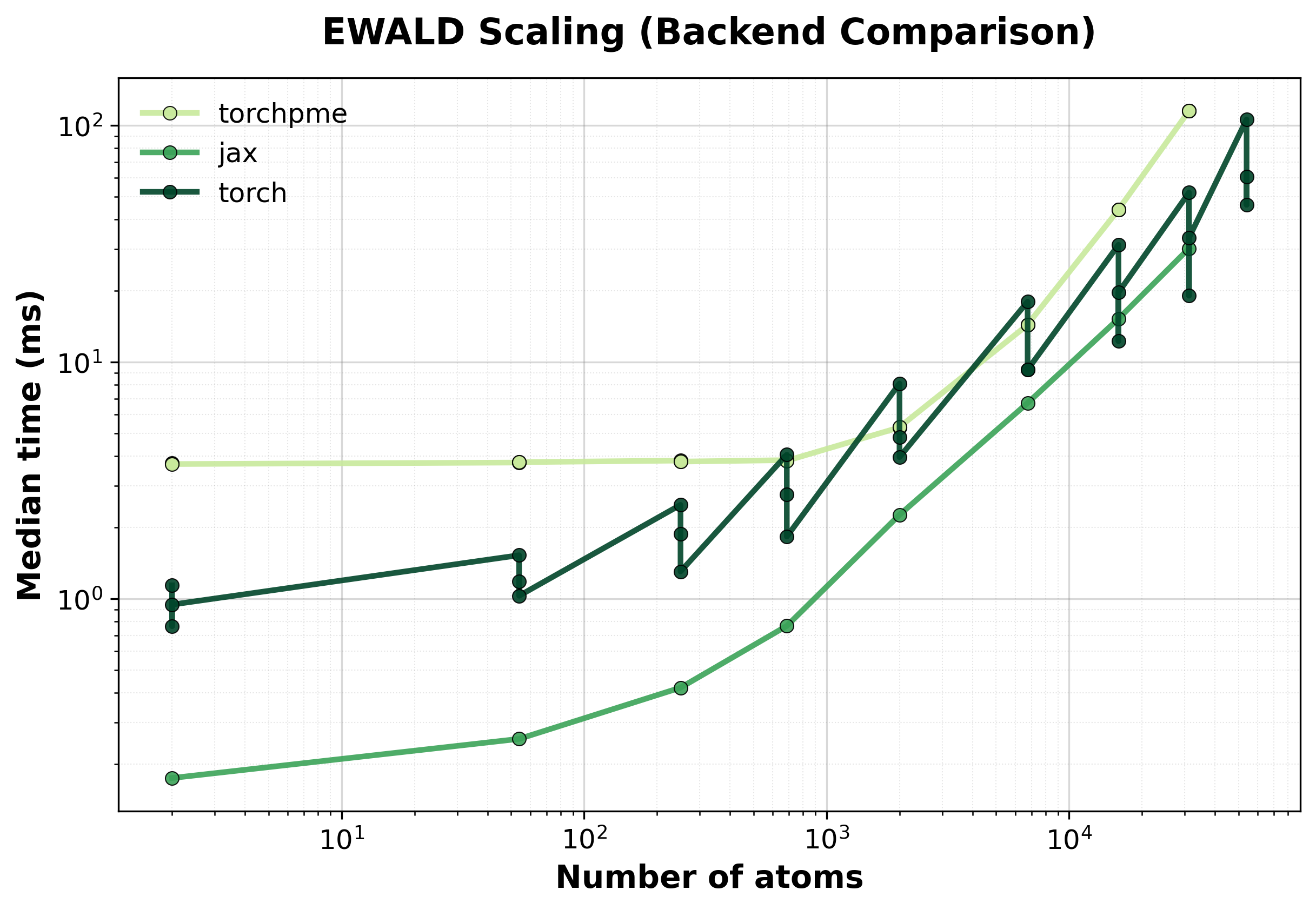
Median execution time comparison between backends for single systems.

Throughput

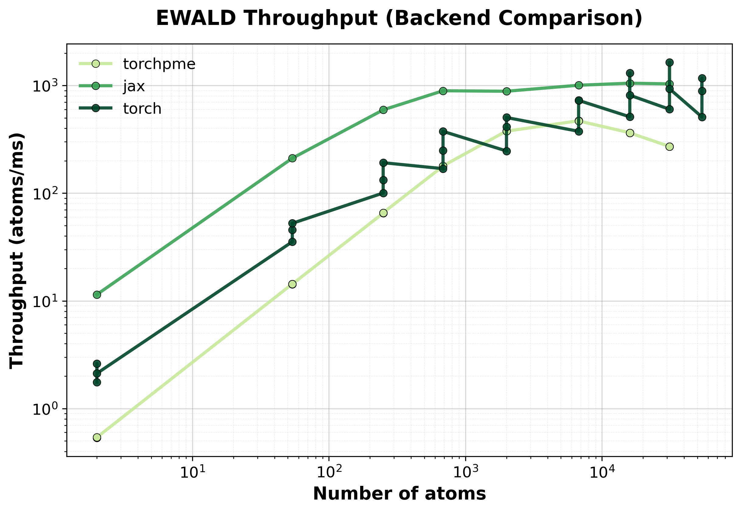
Throughput (atoms/ms) comparison between backends. Higher values indicate better performance.

Memory Usage

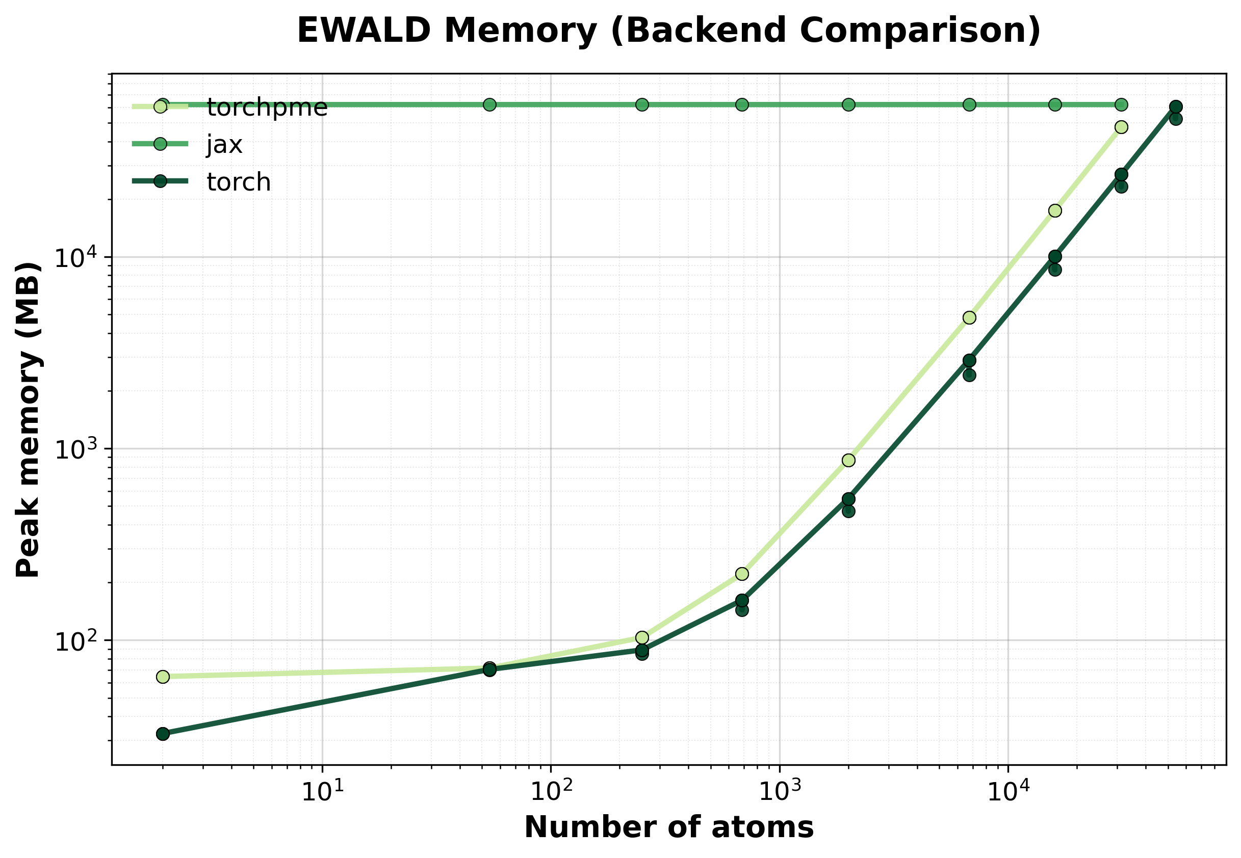
Peak GPU memory consumption comparison between backends. Lower is better, indicating that the backend has lower memory requirements.

nvalchemiops (Torch)

Scaling of single and batched Ewald computation with the nvalchemiops Torch backend. Shows how performance scales with different batch sizes.

Time Scaling

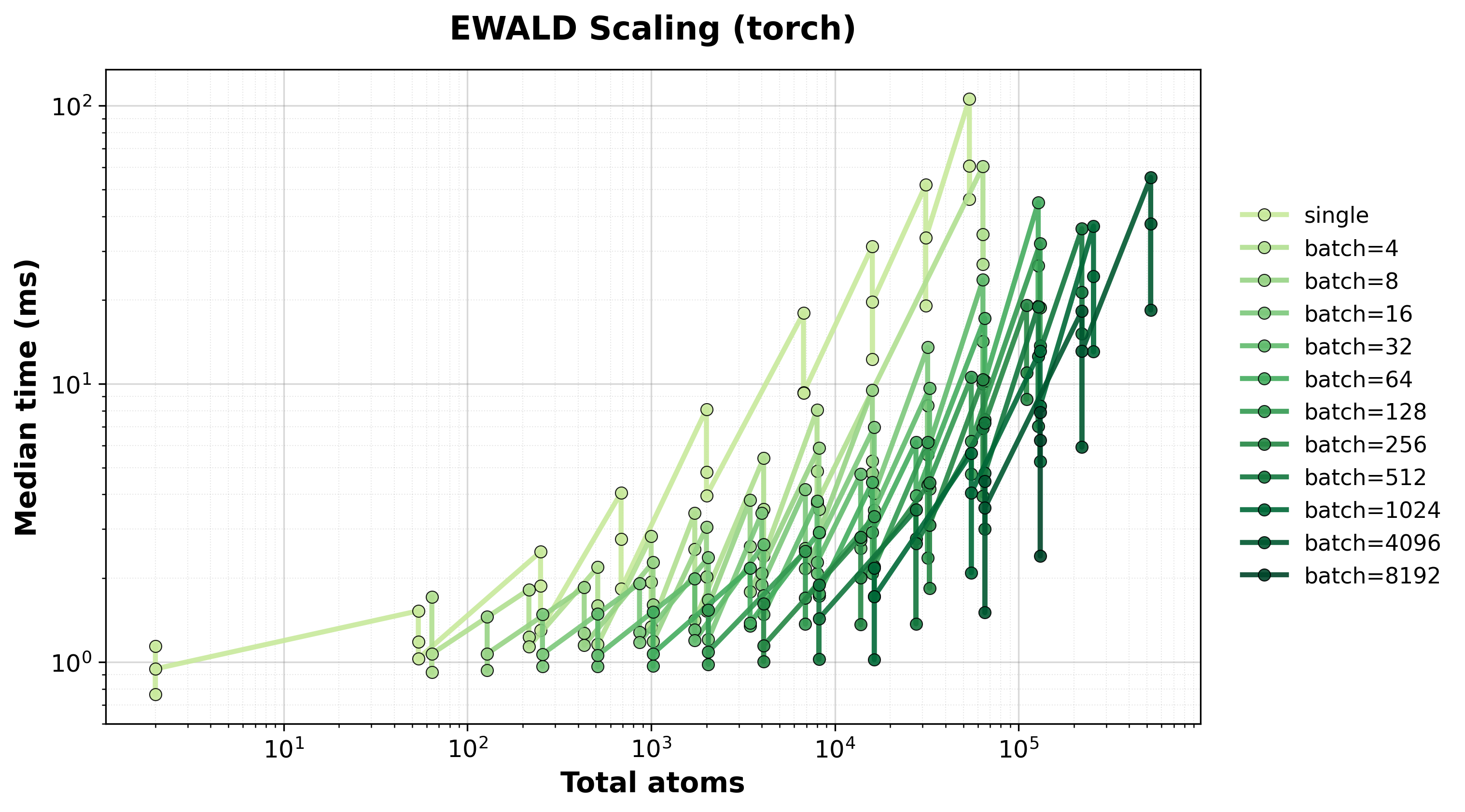
Execution time scaling for single and batched systems.

Throughput

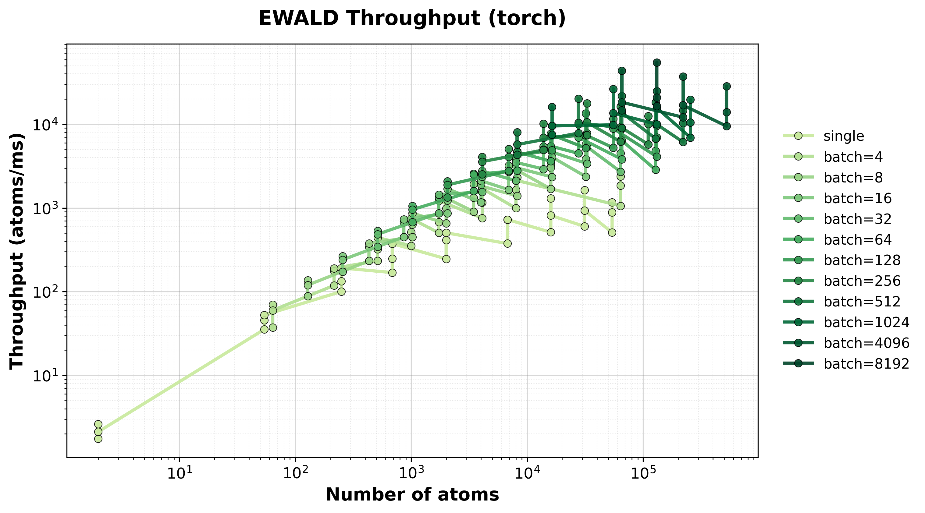
Throughput (atoms/ms) for single and batched systems.

Memory Usage

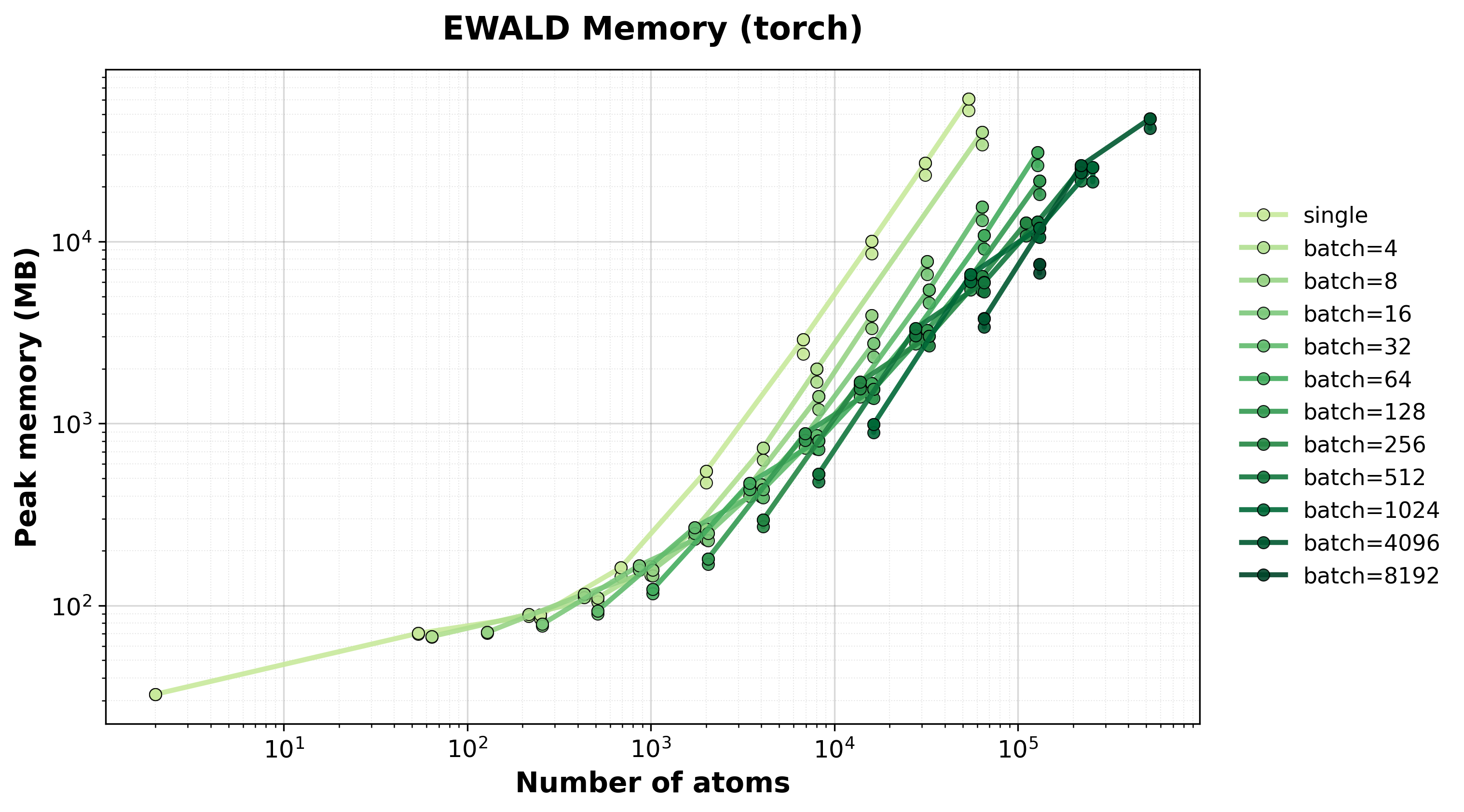
Peak GPU memory consumption for single and batched systems.

nvalchemiops (JAX)

Scaling of single and batched Ewald computation with the nvalchemiops JAX backend. Shows how performance scales with different batch sizes.

Time Scaling

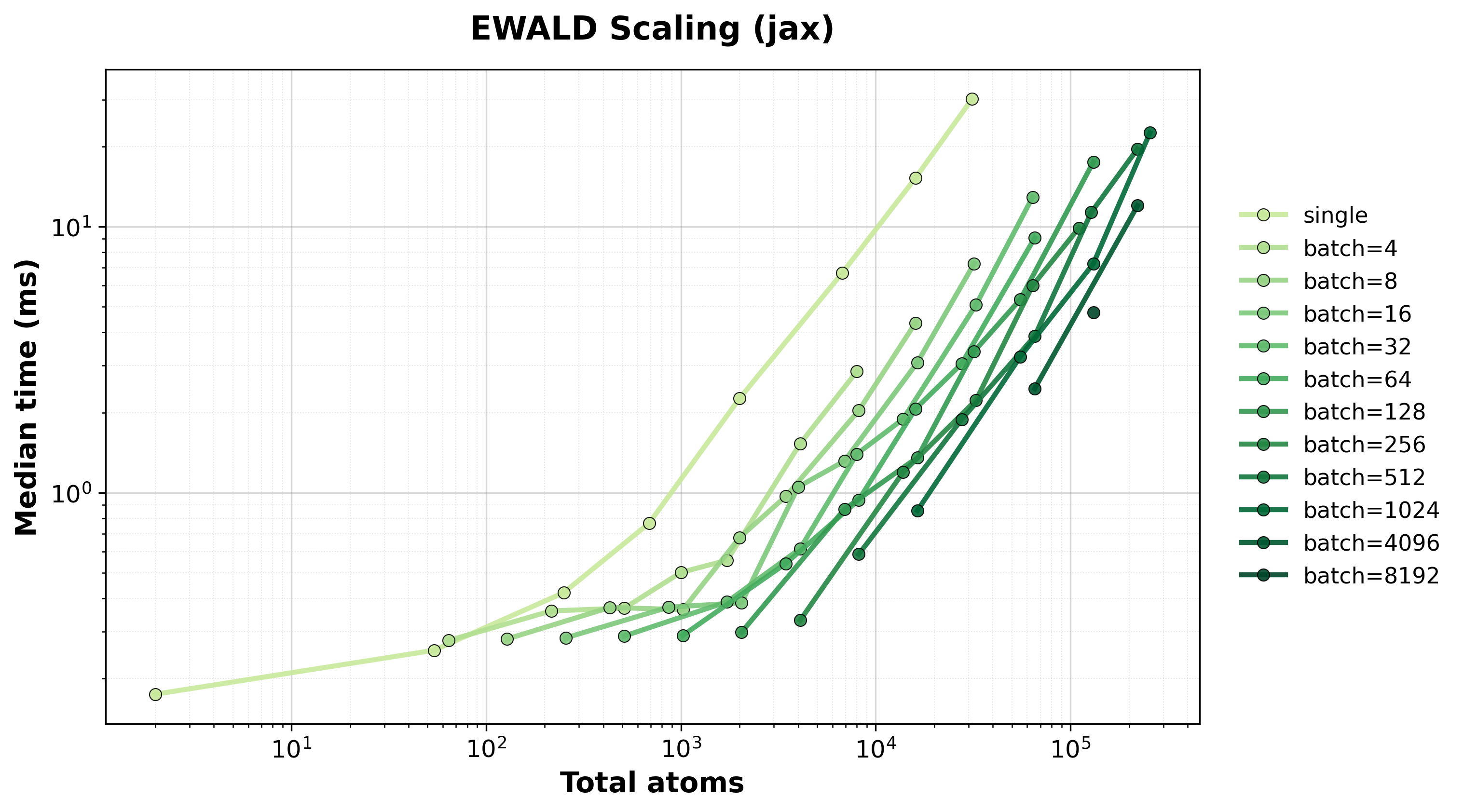
Execution time scaling for single and batched systems.

Throughput

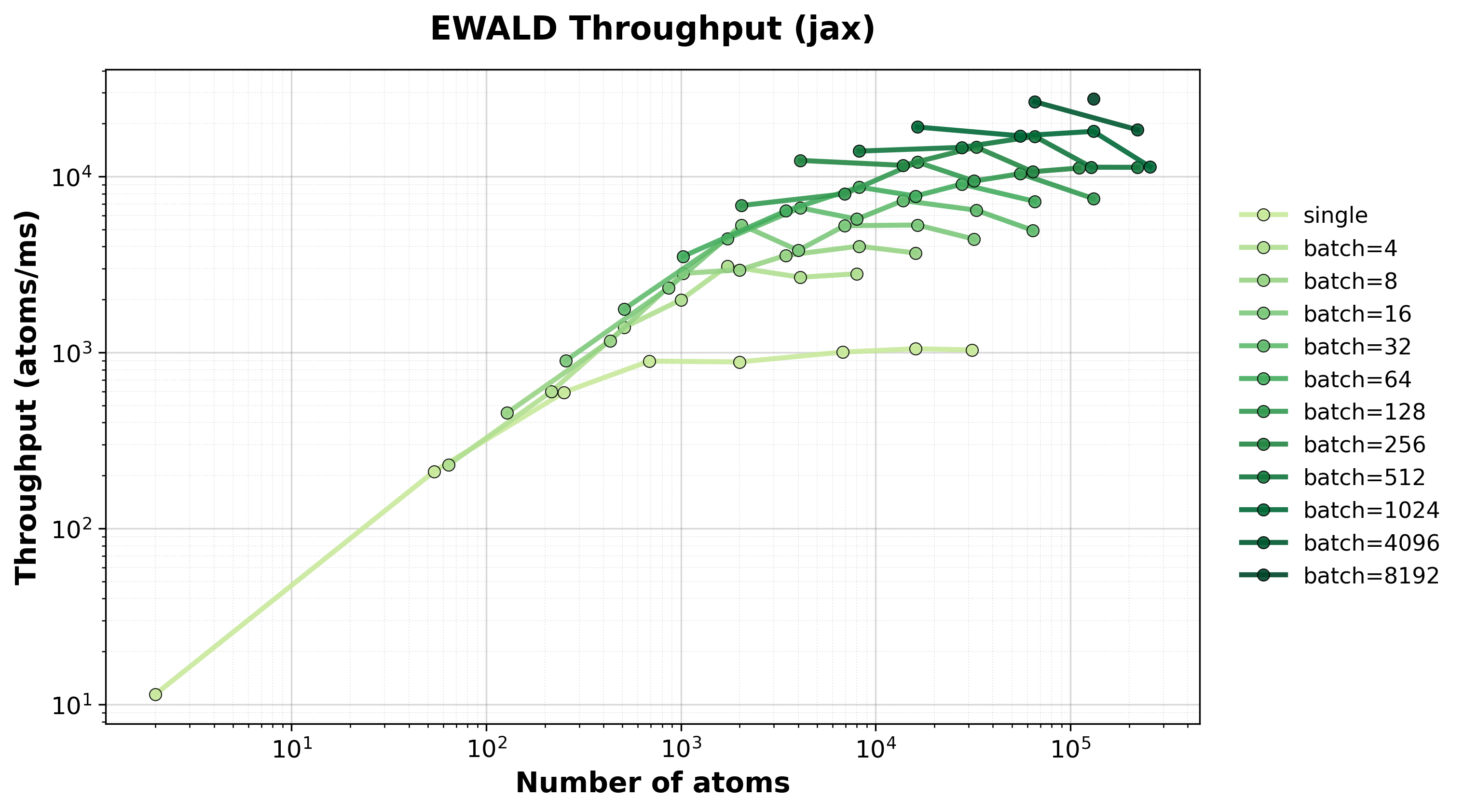
Throughput (atoms/ms) for single and batched systems.

Memory Usage

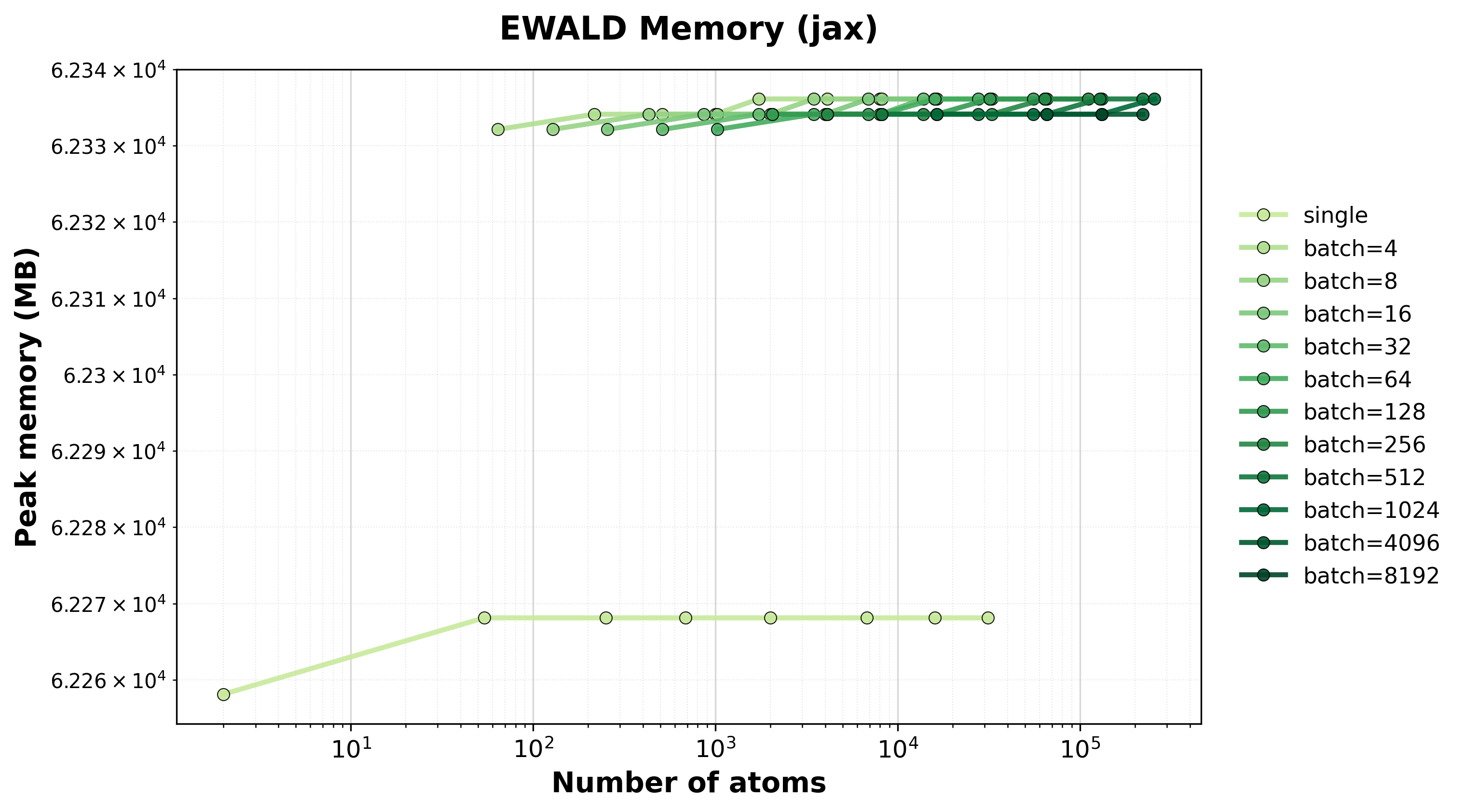
Peak GPU memory consumption for single and batched systems.

Particle Mesh Ewald (PME)

PME achieves \(O(N \log N)\) scaling by using FFTs for the reciprocal-space contribution. This is the recommended method for large systems.

Backend Comparison

Simple comparison of single (non-batched) system computations between backends, where we scale up the size of the supercell.

Time Scaling

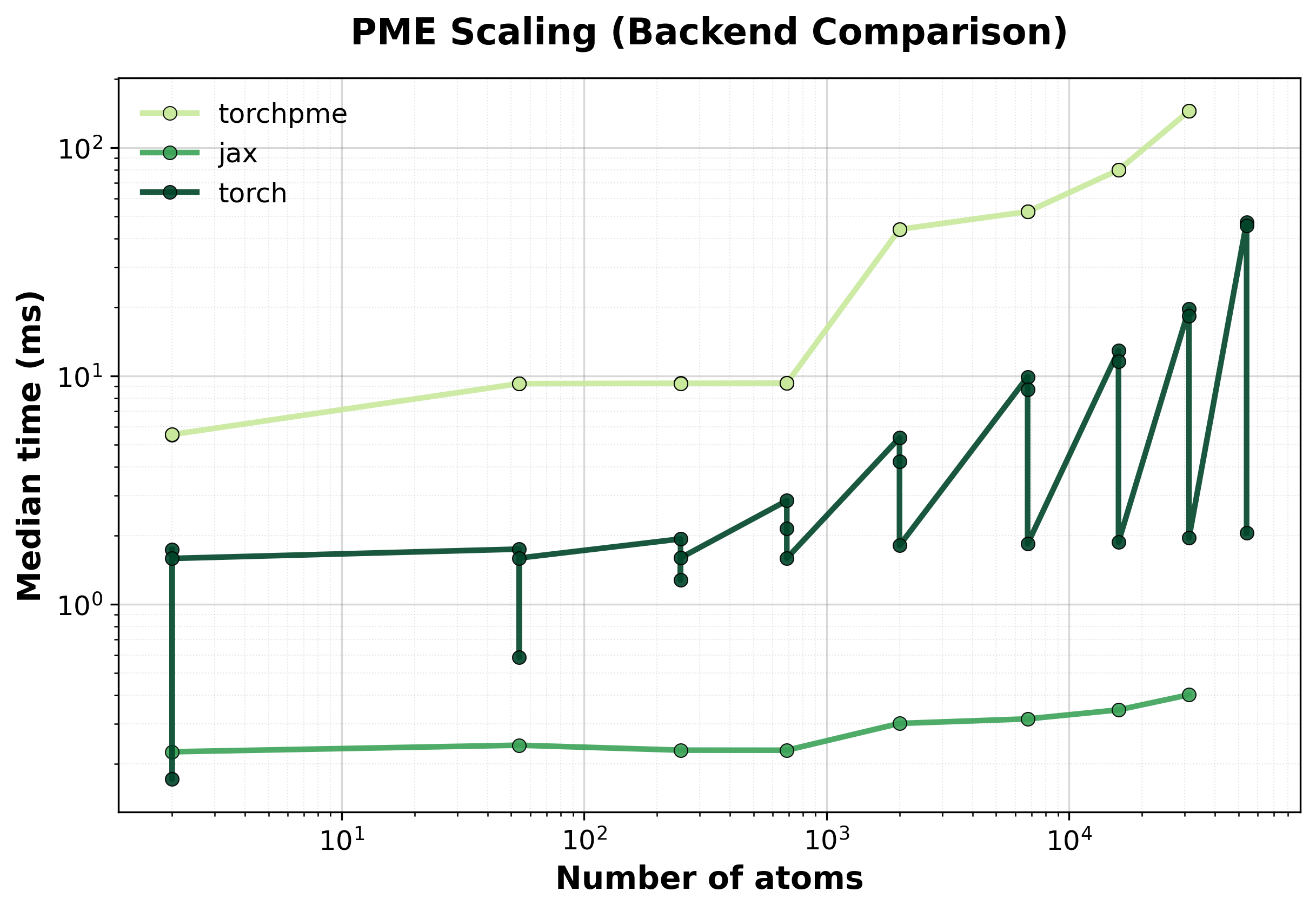
Median execution time comparison between backends for single systems.

Throughput

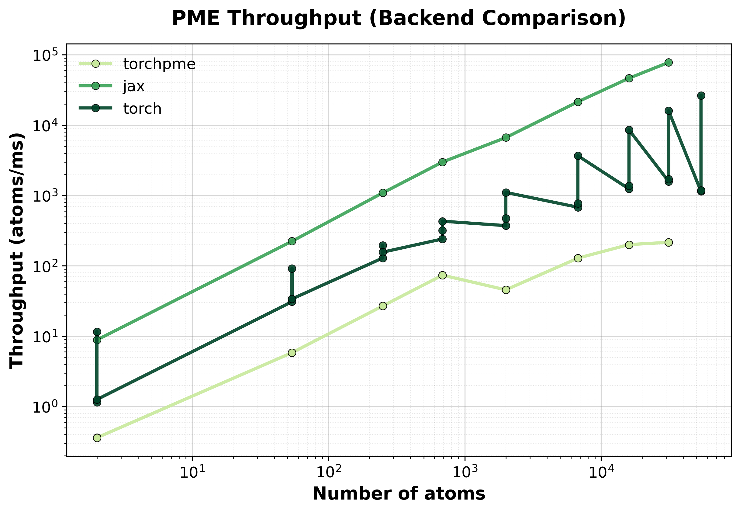
Throughput (atoms/ms) comparison between backends. Higher values indicate better performance.

Memory Usage

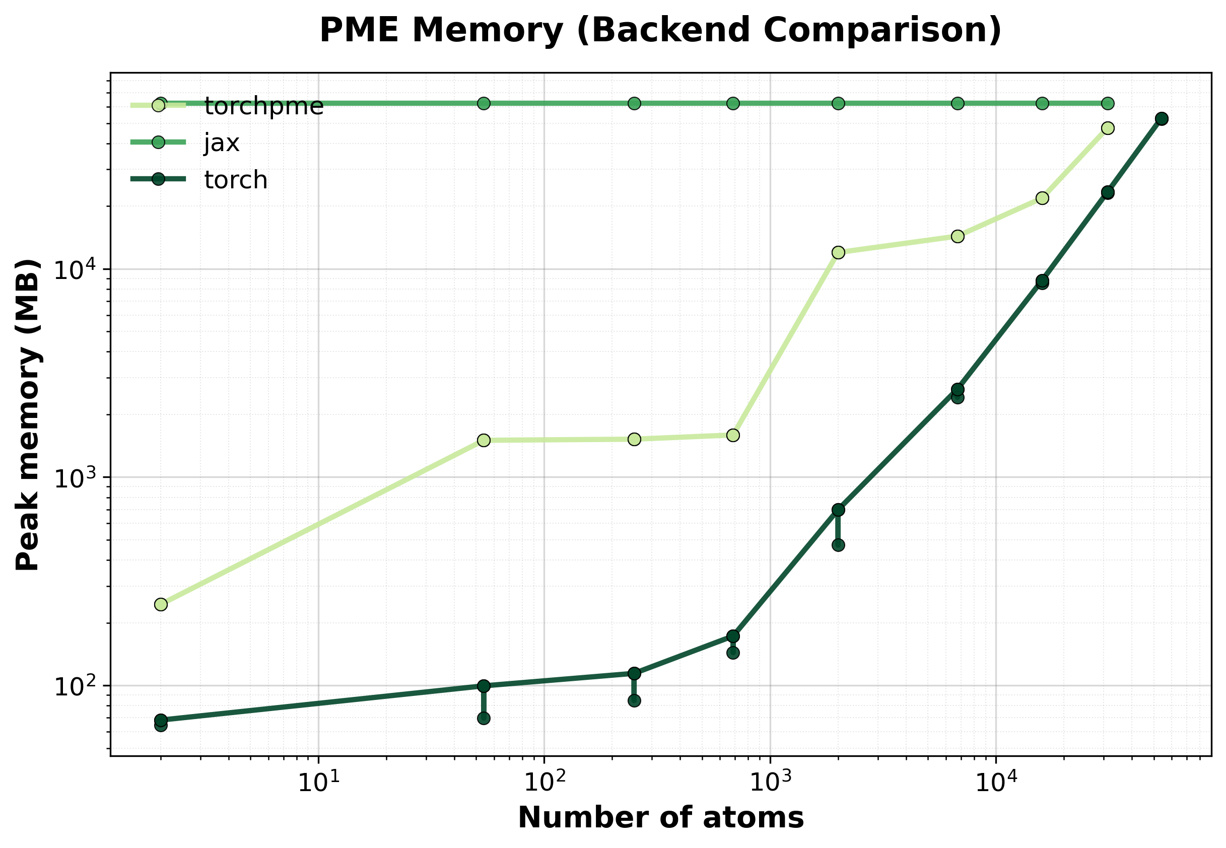
Peak GPU memory consumption comparison between backends. Lower is better, indicating that the backend has lower memory requirements.

nvalchemiops (Torch)

Scaling of single and batched PME computation with the nvalchemiops Torch backend. Shows how performance scales with different batch sizes.

Time Scaling

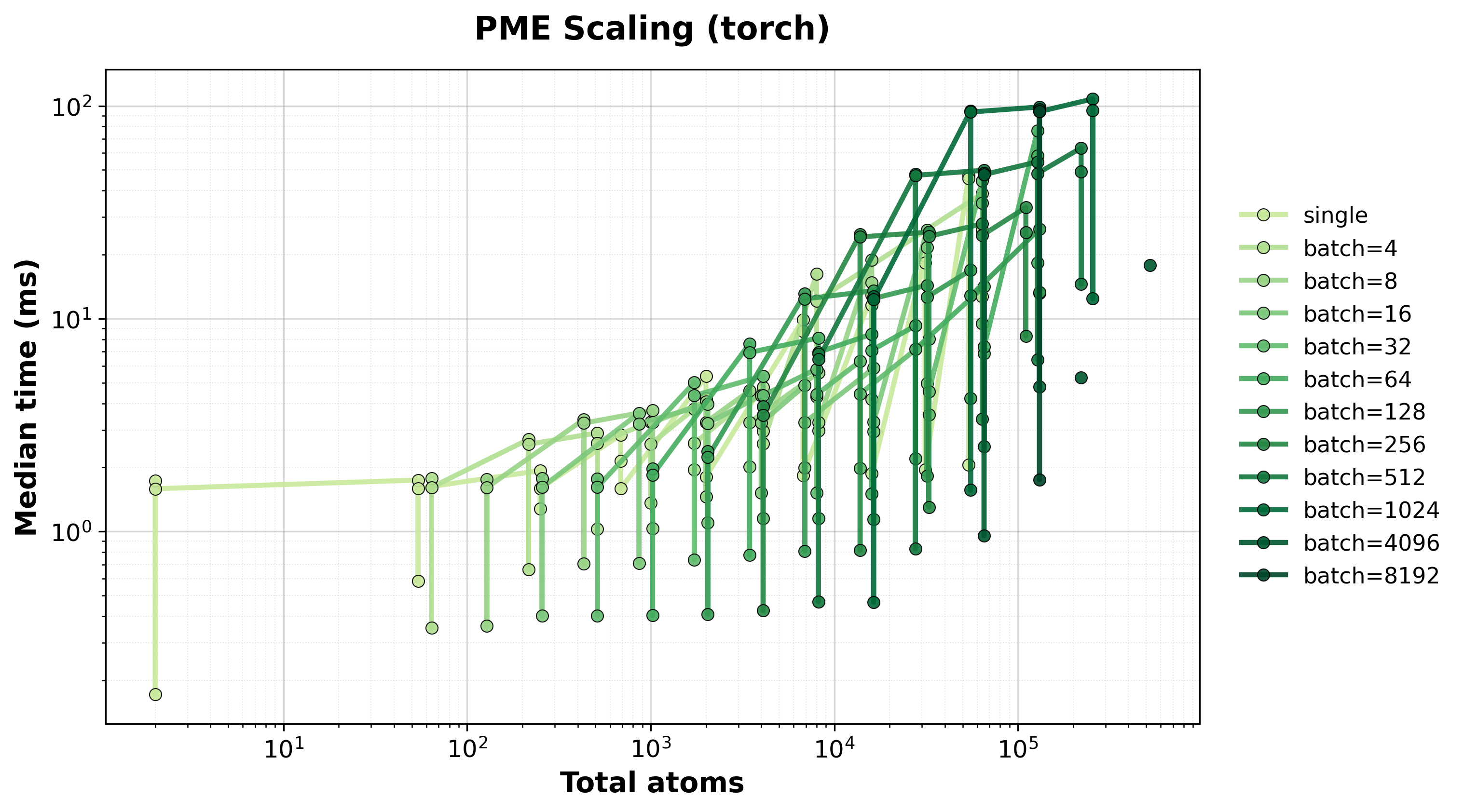
Execution time scaling for single and batched systems.

Throughput

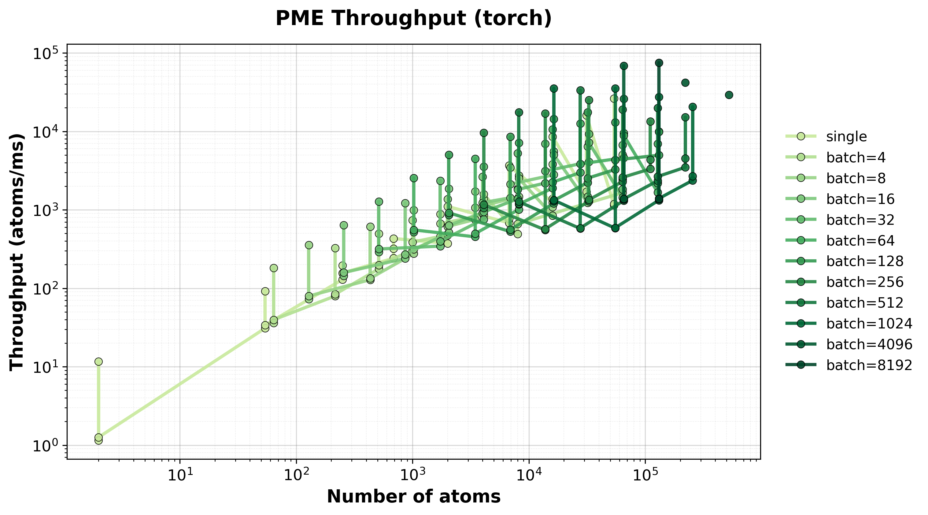
Throughput (atoms/ms) for single and batched systems.

Memory Usage

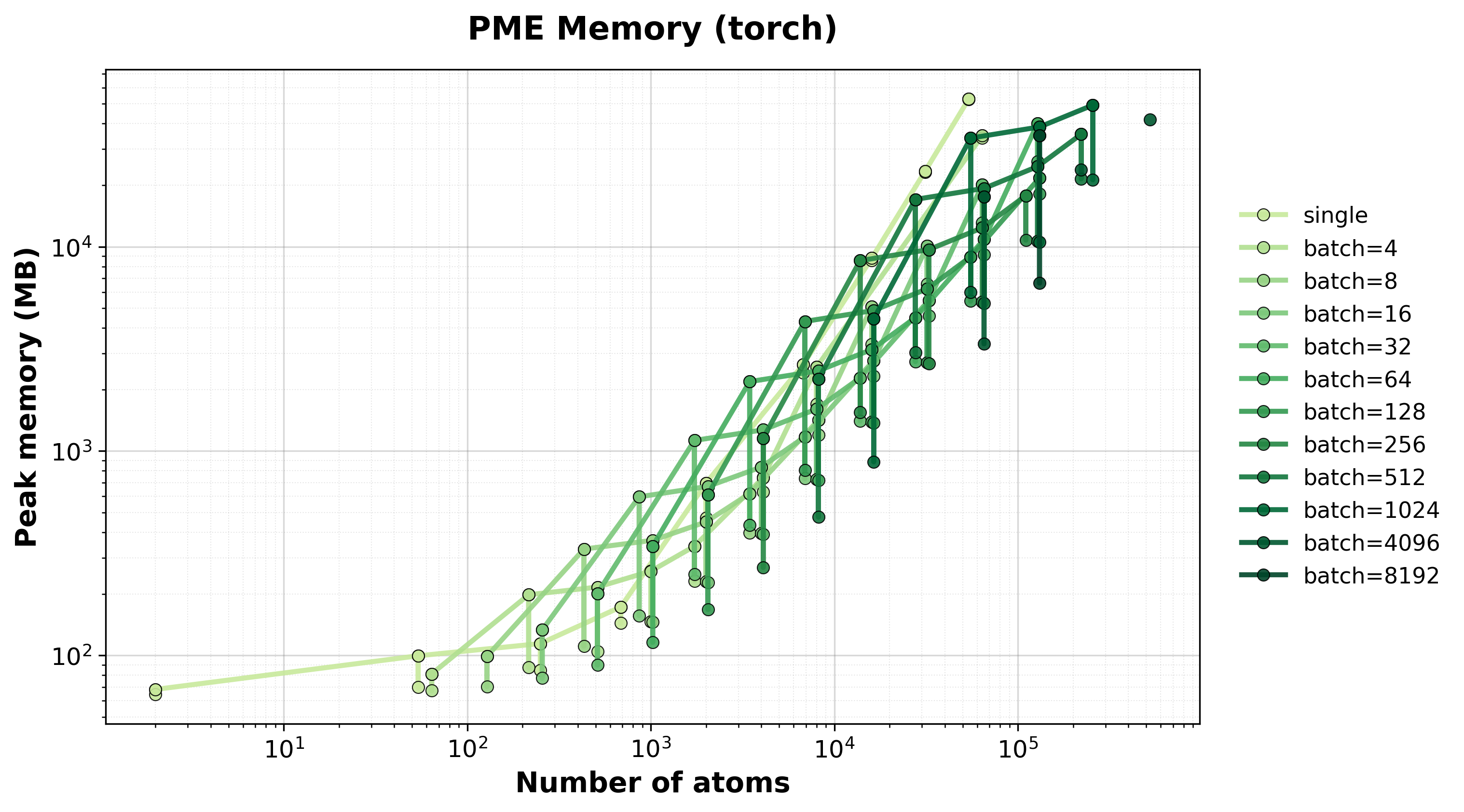
Peak GPU memory consumption for single and batched systems.

nvalchemiops (JAX)

Scaling of single and batched PME computation with the nvalchemiops JAX backend. Shows how performance scales with different batch sizes.

Time Scaling

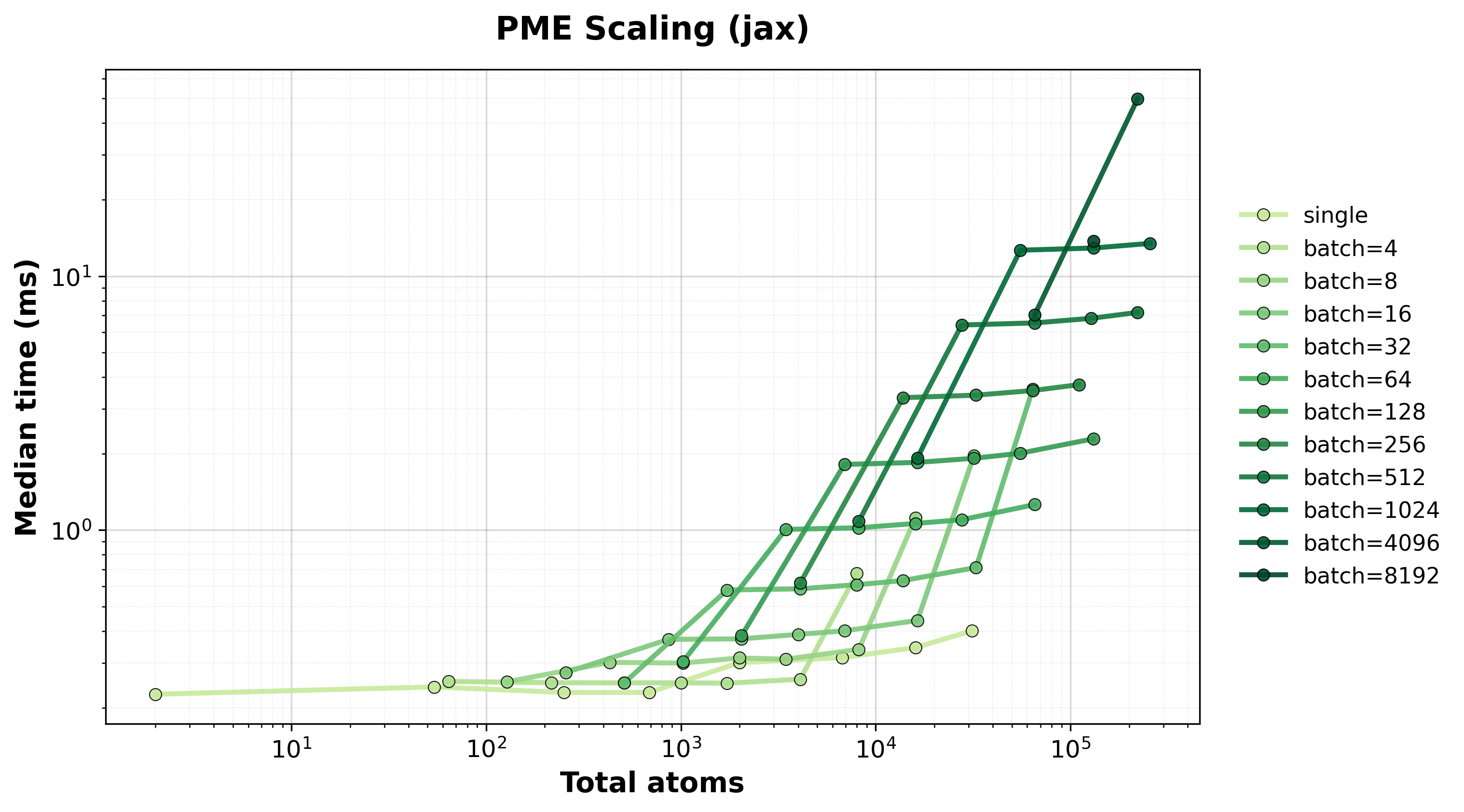
Execution time scaling for single and batched systems.

Throughput

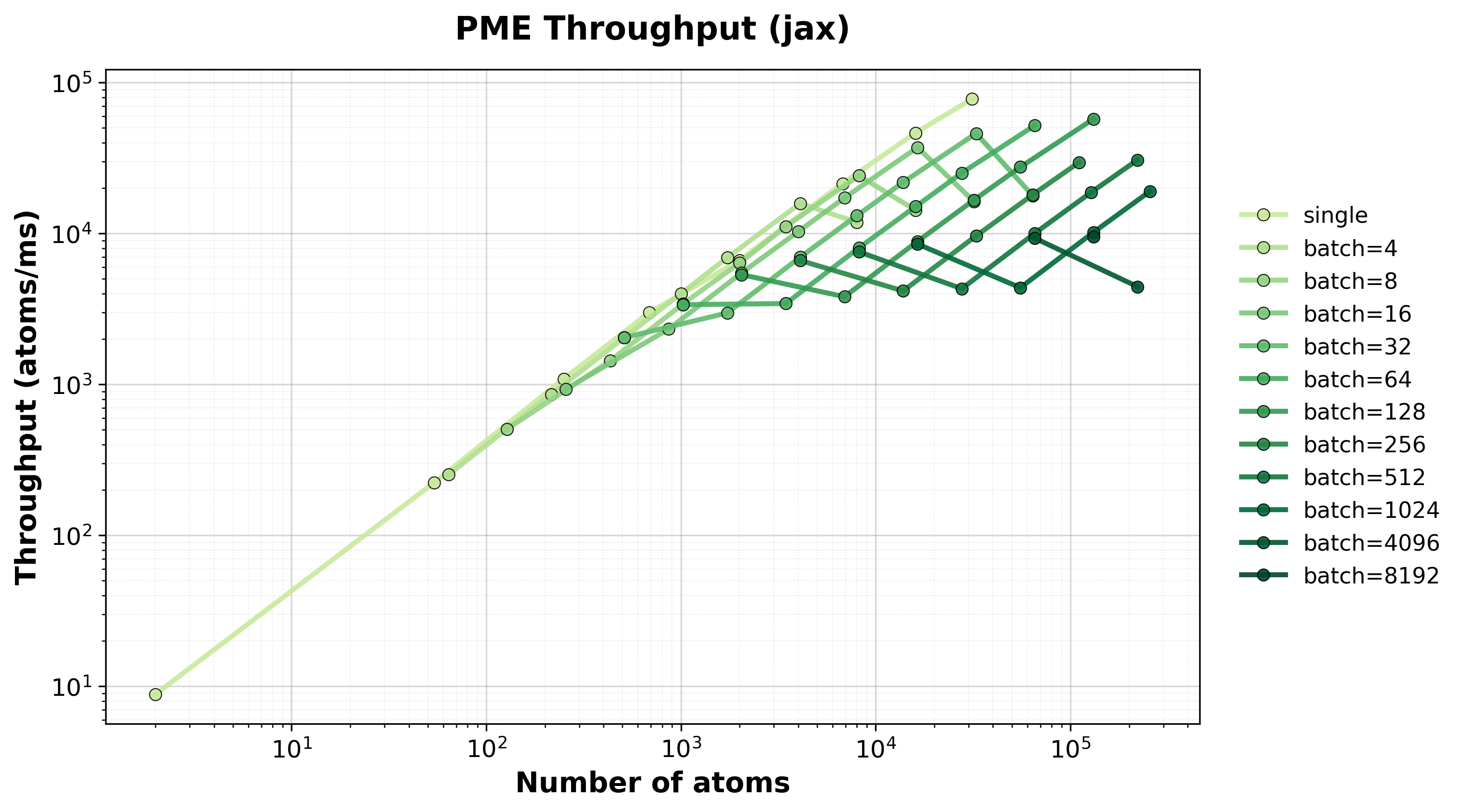
Throughput (atoms/ms) for single and batched systems.

Memory Usage

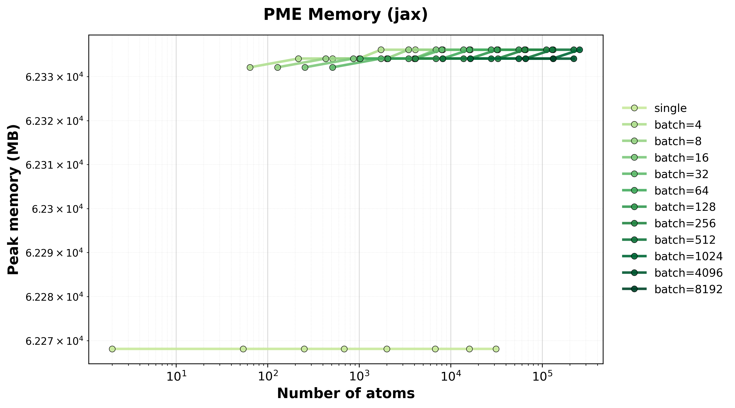
Peak GPU memory consumption for single and batched systems.

Damped Shifted Force (DSF)

The DSF method is a purely real-space, pairwise \(O(N)\) electrostatic summation. Unlike Ewald and PME, DSF has no reciprocal-space component – benchmarks measure the full calculation directly. DSF supports both CSR neighbor list and dense neighbor matrix formats, and can be compared against a pure PyTorch reference implementation (torch_dsf backend).

Note

DSF benchmark plots will be added in a future update. Performance and accuracy benchmark scripts are available in benchmarks/interactions/electrostatics/ and can be run on your hardware using the instructions below.

DSF Parameters

Parameter	Value
cutoff	12.0
alpha	0.2
component	full (real-space only, no reciprocal-space split)

Hardware Information

GPU: NVIDIA H100 80GB HBM3

Benchmark Configuration

Parameter	Value
System Type	FCC crystal lattice with periodic boundaries
Neighbor List	Cell list algorithm (\(O(N)\) scaling)
Warmup Iterations	3
Timing Iterations	10
Precision	float32

Ewald/PME Parameters

Parameters are automatically estimated using accuracy-based parameter estimation targeting \(10^{-6}\) relative accuracy:

Parameter	Description
alpha	Ewald splitting parameter (auto-estimated)
k_cutoff	Reciprocal-space cutoff for Ewald (auto-estimated)
real_space_cutoff	Real-space cutoff distance (auto-estimated)
mesh_dimensions	PME mesh grid size (auto-estimated)
spline_order	B-spline interpolation order (4)

Interpreting Results

total_atoms : Total number of atoms in the supercell (or across all batched systems).

batch_size : Number of systems processed simultaneously (1 for single-system mode).

method : The electrostatics method used (ewald, pme, or dsf).

backend : The computational backend (torch, jax, torchpme, or torch_dsf).

component : Which part of the calculation was benchmarked (real, reciprocal, or full).

compute_forces : Whether forces were computed in addition to energies.

median_time_ms : Median execution time in milliseconds (lower is better).

peak_memory_mb : Peak GPU memory usage in megabytes.

Note

Timings include the full electrostatics calculation (real-space + reciprocal-space for “full” mode). Neighbor list construction is excluded from timings.

Running Your Own Benchmarks

To generate benchmark results for your hardware:

torch Backend (default)

cd benchmarks/interactions/electrostatics
python benchmark_electrostatics.py \
    --config benchmark_config.yaml \
    --backend torch \
    --method all \
    --output-dir ../../../docs/benchmarks/benchmark_results

jax Backend

cd benchmarks/interactions/electrostatics
python benchmark_electrostatics.py \
    --config benchmark_config.yaml \
    --backend jax \
    --method both \
    --output-dir ../../../docs/benchmarks/benchmark_results

torchpme Backend

cd benchmarks/interactions/electrostatics
python benchmark_electrostatics.py \
    --config benchmark_config.yaml \
    --backend torchpme \
    --method both \
    --output-dir ../../../docs/benchmarks/benchmark_results

Options

--backend {torch,jax,torchpme,torch_dsf,both} : Computational backend (default: torch). both dispatches per-method: torch + torchpme for Ewald/PME, torch + torch_dsf for DSF.

--method {ewald,pme,dsf,both,all} : Electrostatics method (default: both). both = Ewald + PME (backward compatible). all = Ewald + PME + DSF.

--neighbor-format {list,matrix,both} : Neighbor format for DSF benchmarks (default: list). Ewald/PME always use matrix.

--dtype {float32,float64} : Override dtype from config file.

--gpu-sku <name> : Override GPU SKU name for output files (default: auto-detect).

--config <path> : Path to YAML configuration file.

DSF-Only Benchmark

python benchmark_electrostatics.py \
    --config benchmark_config.yaml \
    --backend both \
    --method dsf \
    --neighbor-format list

Results will be saved as CSV files and plots will be automatically generated during the next documentation build.