ModelNet40 Classification

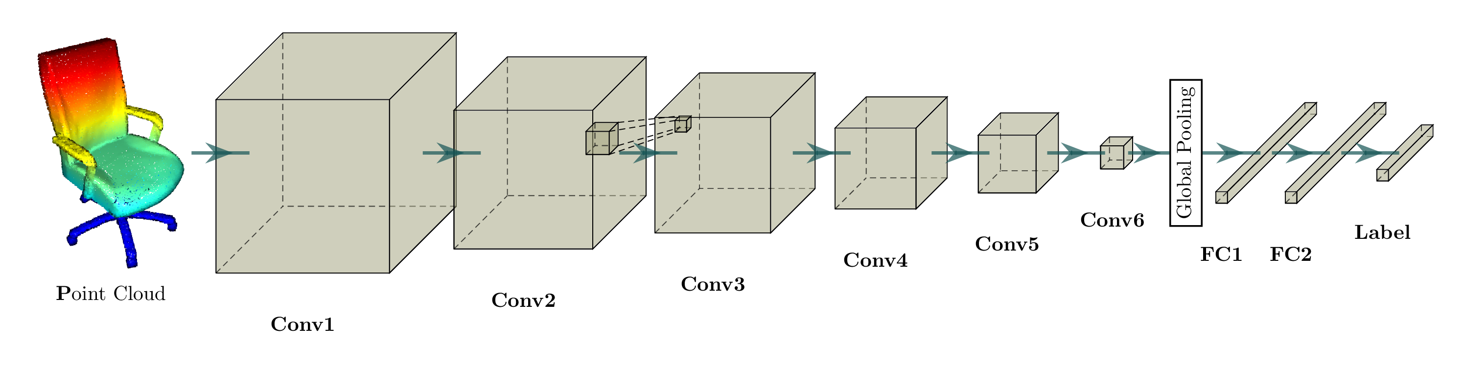
In this page, we will go over a simple demo example that trains a 3D convolutional neural network with for classification. The input is a sparse tensor and convolution is defined on a sparse tensor as well. The network is an extension of the following architecture, but with residual blocks and a lot more layers.

Before we proceed, please go over the training and data loading tutorial first.

Making a ModelNet40 data loader

First, we need to create a data loader that return a sparse tensor representation of a mesh. However, a mesh representation of a 3D model can be sparse if we only use vertices.

We will first sample points with the same density.

def resample_mesh(mesh_cad, density=1):
    '''
    https://chrischoy.github.io/research/barycentric-coordinate-for-mesh-sampling/
    Samples point cloud on the surface of the model defined as vectices and
    faces. This function uses vectorized operations so fast at the cost of some
    memory.

    param mesh_cad: low-polygon triangle mesh in o3d.geometry.TriangleMesh
    param density: density of the point cloud per unit area
    param return_numpy: return numpy format or open3d pointcloud format
    return resampled point cloud

    Reference :
      [1] Barycentric coordinate system
      \begin{align}
        P = (1 - \sqrt{r_1})A + \sqrt{r_1} (1 - r_2) B + \sqrt{r_1} r_2 C
      \end{align}
    '''
    faces = np.array(mesh_cad.triangles).astype(int)
    vertices = np.array(mesh_cad.vertices)

    vec_cross = np.cross(vertices[faces[:, 0], :] - vertices[faces[:, 2], :],
                         vertices[faces[:, 1], :] - vertices[faces[:, 2], :])
    face_areas = np.sqrt(np.sum(vec_cross**2, 1))

    n_samples = (np.sum(face_areas) * density).astype(int)

    n_samples_per_face = np.ceil(density * face_areas).astype(int)
    floor_num = np.sum(n_samples_per_face) - n_samples
    if floor_num > 0:
        indices = np.where(n_samples_per_face > 0)[0]
        floor_indices = np.random.choice(indices, floor_num, replace=True)
        n_samples_per_face[floor_indices] -= 1

    n_samples = np.sum(n_samples_per_face)

    # Create a vector that contains the face indices
    sample_face_idx = np.zeros((n_samples,), dtype=int)
    acc = 0
    for face_idx, _n_sample in enumerate(n_samples_per_face):
        sample_face_idx[acc:acc + _n_sample] = face_idx
        acc += _n_sample

    r = np.random.rand(n_samples, 2)
    A = vertices[faces[sample_face_idx, 0], :]
    B = vertices[faces[sample_face_idx, 1], :]
    C = vertices[faces[sample_face_idx, 2], :]

    P = (1 - np.sqrt(r[:, 0:1])) * A + \
        np.sqrt(r[:, 0:1]) * (1 - r[:, 1:]) * B + \
        np.sqrt(r[:, 0:1]) * r[:, 1:] * C

    return P

The above function will sample points on a mesh with the same density. Next, we go through a series of data augmentation steps before quantization steps.

Data Augmentation

A sparse tensor consists of two components: 1) coordinates and 2) features associated to those coordinates. We have to apply data augmentation to both components to maximize the utility of the fixed dataset and make the network robust to noise.

This is nothing new in image data-augmentation. We apply random translation, shear, scaling to an image, all of which are coordinate data-augmentation. Color distortions such as chromatic translation, Gaussian noise on color channels, hue-saturation augmentations are all feature data-augmentation.

However, since we have only coordinates as data in the ModelNet40 dataset, we will only apply coordinate data-augmentation.

class RandomRotation:

    def _M(self, axis, theta):
        return expm(np.cross(np.eye(3), axis / norm(axis) * theta))

    def __call__(self, coords, feats):
        R = self._M(
            np.random.rand(3) - 0.5, 2 * np.pi * (np.random.rand(1) - 0.5))
        return coords @ R, feats


class RandomScale:

    def __init__(self, min, max):
        self.scale = max - min
        self.bias = min

    def __call__(self, coords, feats):
        s = self.scale * np.random.rand(1) + self.bias
        return coords * s, feats


class RandomShear:

    def __call__(self, coords, feats):
        T = np.eye(3) + np.random.randn(3, 3)
        return coords @ T, feats


class RandomTranslation:

    def __call__(self, coords, feats):
        trans = 0.05 * np.random.randn(1, 3)
        return coords + trans, feats

Training a ResNet for ModelNet40 Classification

The main training function is simple. However, instead of epoch-based training, I used iteration-based training. One advantage of iteration-based training over the epoch-based training is that the training logic is independent of the batch-size.

def train(net, device, config):
    optimizer = optim.SGD(
        net.parameters(),
        lr=config.lr,
        momentum=config.momentum,
        weight_decay=config.weight_decay)
    scheduler = optim.lr_scheduler.ExponentialLR(optimizer, 0.95)

    crit = torch.nn.CrossEntropyLoss()

   ...

    net.train()
    train_iter = iter(train_dataloader)
    val_iter = iter(val_dataloader)
    logging.info(f'LR: {scheduler.get_lr()}')
    for i in range(curr_iter, config.max_iter):

        s = time()
        data_dict = train_iter.next()
        d = time() - s

        optimizer.zero_grad()
        sin = ME.SparseTensor(data_dict['feats'],
                              data_dict['coords'].int()).to(device)
        sout = net(sin)
        loss = crit(sout.F, data_dict['labels'].to(device))
        loss.backward()
        optimizer.step()
        t = time() - s

        ...

Running the Example

When you assemble all the code blocks, you can run your own ModelNet40 classification network.

python -m examples.modelnet40 --batch_size 128 --stat_freq 100

The entire code can be found at example/modelnet40.py.

Warning

The ModelNet40 data loading and voxelization is the most time consuming part of the training. Thus, the example caches all ModelNet40 data into memory which takes up about 10G of memory.