Tacotron 2
Model
This model is based on the Tacotron 2 model (see also paper). Our implementation mostly matches what is presented in the paper. There are a few differences listed below.
The biggest change from Tacotron 2 is that in addition to supporting the
generation of mel spectrograms, we support generating magnitude/energy
spectrograms as well. This is controlled via the output_type variable inside
the config file. output_type = "mel" matches the paper minus the differences
below. output_type = "magnitude" matches the paper with the difference that
the output spectrogram is a magnitude spectrogram as opposed to mel. output_type = "both"
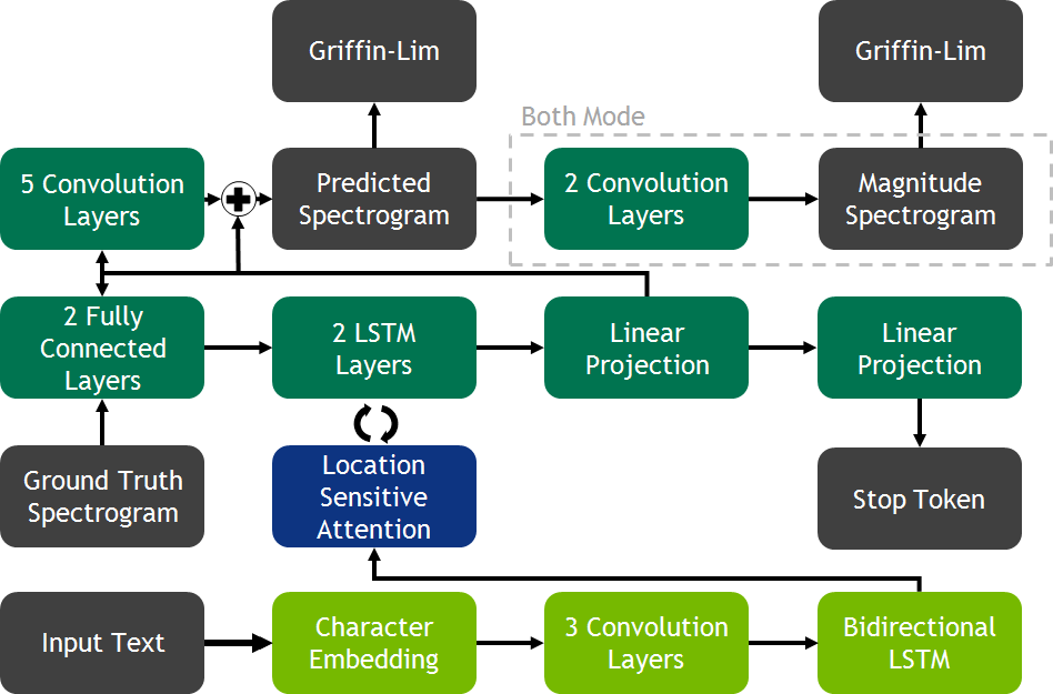
matches output_type = "mel" with the addition of 2 convolutional layers
that learns a mapping from a log mel spectrogram to a magnitude spectrogram.
This is the architecture shown in the picture below.
The second change is the location of the stop token linear projection layer. In the paper, it is connected to the output of the decoder rnn. Whereas in our implementation, it is connected to the output of the spectrogram projection layer.
We replace zoneout with dropout in the decoder rnn and remove it entirely from the encoder rnn.
Lastly, the convolutional layer used inside the location layer of the attention has a kernel size of 32 as opposed to 31 as stated in the tacotron 2 paper.
Model Description
Tacotron 2 Model
Tacotron 2 follows a simple encoder decoder structure that has seen great success in sequence-to-sequence modeling. The encoder is made of three parts. First a word embedding is learned. The embedding is then passed through a convolutional prenet. Lastly, the results are consumed by a bi-direction rnn. The encoder and decoder structure is connected via an attention mechanism which the Tacotron authors refer to as Location Sensitive Attention and is described in Attention-Based Models for Speech Recognition. The decoder is comprised of a 2 layer LSTM network, a convolutional postnet, and a fully connected prenet. During training, the ground frame is fed through the prenet and passed as input to the LSTM layers. In addition, an attention context is computed by the attention layer at each step and concatenated with the prenet output. The output of the LSTM network concatenated with the attention is sent through two projection layers. The first projects the information to a spectrogram while the other projects it to a stop token. The spectrogram is then sent through the convolutional postnet to compute a residual to add to the generated spectrogram. The addition of the generated spectrogram and the residual results in a final spectrogram that is used to generate speech using Griffin-Lim.
If using the default both mode, the final mel spectrogram is sent through additional convolutional layers to learn a mapping from the log mel spectrogram to a magnitude spectrogram. The learned magnitude spectrogram is then sent through Griffin-Lim.
Training
The model is trained with ADAM with an initial learning rate of 1e-3 with an exponential decay that starts at 45k steps. The learning rate decays at a rate of 0.1 every 20k steps until 85k when it reaches the minimum learning rate of 1e-5.
The model is regularized using l2 regularization with a weight of 1e-6.
Tips and Tricks
A pseudo metric for audio quality is how well attention is learned. Ideally, we want a nice clear diagonal alignment. The current models should learn attention between 10k - 20k steps.
It seems that dropout is just as effective as zoneout when training. Since dropout is faster during training then zoneout, we have decided to switch to dropout.