GEMM Profiling Tutorial
This tutorial shows how to go from a transformer model config to concrete GEMM shapes, benchmark them across precisions (BF16, FP8 CurrentScaling, FP8 DelayedScaling, FP8 Block, MXFP8, NVFP4), and compute expected speedups. If you are using NVIDIA Transformer Engine – which handles the quantization and kernel dispatch for these precision modes – this is how you derive the matrix multiplications your model runs and measure where your time goes.
The benchmark tool is at benchmarks/gemm/benchmark_gemm.py.
Quick Start: Model Config Mode
The benchmark tool takes model hyperparameters directly and handles everything – deriving GEMM shapes, benchmarking across precisions, and computing the full speedup analysis – in a single command:
python benchmarks/gemm/benchmark_gemm.py \
  --hidden_size 4096 \
  --intermediate_size 16384 \
  --num_attention_heads 32 \
  --num_hidden_layers 24 \
  --micro_batch_size 31 \
  --sequence_length 512 \
  -o ./gemm_speedup.png
On Hopper (H100/H200), skip MXFP8 and NVFP4 which require Blackwell:
python benchmarks/gemm/benchmark_gemm.py \
  --hidden_size 4096 \
  --intermediate_size 16384 \
  --num_attention_heads 32 \
  --num_hidden_layers 24 \
  --micro_batch_size 31 \
  --sequence_length 512 \
  --no-fp8 --no-fp4 \
  -o ./gemm_speedup.png
By default the tool runs in autocast mode, which is what Transformer Engine does during training: inputs are dynamically quantized to the target precision before each GEMM, so the measured time includes both the quantization cost and the GEMM kernel itself. This gives the realistic end-to-end picture.
The tool computes M = 31 x 512 = 15,872 tokens, derives all 12 GEMM shapes
(4 Fprop + 4 Dgrad + 4 Wgrad), benchmarks each across enabled precisions, and prints
the full results. Fprop, Dgrad, and Wgrad shapes are all benchmarked separately to
capture the impact of different matrix aspect ratios on kernel selection.
GEMM Benchmark (Model Config Mode) on NVIDIA B300 SXM6 AC
Timing method: CUDA events
Warmup iterations: 10, Timed iterations: 100
Mode: Autocast (includes quantization overhead)

==========================================================================================
Model Config: hidden=4096, intermediate=16384, heads=32, layers=24
Tokens per step: M = 31 x 512 = 15,872
==========================================================================================

Fprop Shapes:
------------------------------------------------------------------------------------------
Op                     Shape                       BF16 ms FP8Current ms FP8Delayed ms   MXFP8 ms   NVFP4 ms
------------------------------------------------------------------------------------------
QKV Proj               15872x4096x12288              1.071      0.605      0.503      0.579      0.392
Attn Out               15872x4096x4096               0.307      0.317      0.231      0.269      0.256
MLP Up                 15872x4096x16384              1.393      0.924      0.850      0.924      0.635
MLP Down               15872x16384x4096              1.426      1.033      0.901      1.076      0.649
------------------------------------------------------------------------------------------
Fprop sum (ms):                                     4.196      2.879      2.486      2.847      1.932

==========================================================================================
Per-Layer GEMM Time:
                                  BF16 ms FP8Current ms FP8Delayed ms   MXFP8 ms   NVFP4 ms
Fprop:                              4.196      2.879      2.486      2.847      1.932
Dgrad:                              4.290      3.063      2.621      3.045      2.189
Fprop + Dgrad:                      8.486      5.941      5.107      5.892      4.122
Wgrad:                              4.272      3.205      2.695      3.092      2.331
Per-layer total:                   12.758      9.147      7.802      8.984      6.453

Full Model (24 layers):
Total GEMM time (ms):             306.192    219.522    187.246    215.608    154.869

Estimated GEMM Speedups:
  MXFP8 vs BF16:  1.42x
  NVFP4 vs MXFP8: 1.39x
  NVFP4 vs BF16:  1.98x
==========================================================================================
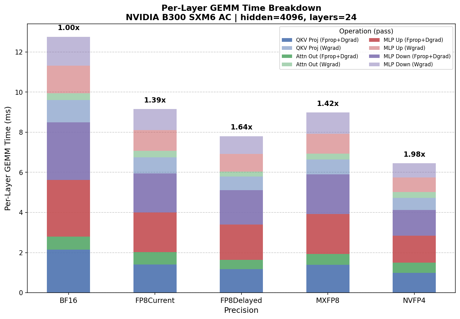
Autocast model config benchmark on NVIDIA B300 – per-layer GEMM time breakdown by precision and operation (Fprop+Dgrad and Wgrad).
Autocast vs Pre-quantized
To isolate raw GEMM kernel performance, add --pre-quantize. This pre-quantizes all
inputs once before the timed loop, so the measured time reflects only the GEMM kernel
execution – no dynamic quantization, no block scaling computation, no format conversion
during the timed region.
Note
FP8 DelayedScaling always runs in autocast mode, even with --pre-quantize,
because it relies on an amax history that requires dynamic quantization. Its
times are therefore not directly comparable to other precisions in pre-quantized
mode.
python benchmarks/gemm/benchmark_gemm.py \
  --hidden_size 4096 \
  --intermediate_size 16384 \
  --num_attention_heads 32 \
  --num_hidden_layers 24 \
  --micro_batch_size 31 \
  --sequence_length 512 \
  --pre-quantize \
  -o ./gemm_speedup_prequant.png
==========================================================================================
Per-Layer GEMM Time:
                                  BF16 ms FP8Current ms FP8Delayed ms   MXFP8 ms   NVFP4 ms
Fprop:                              4.250      2.158      2.555      2.365      1.254
Dgrad:                              4.434      2.329      2.745      2.397      1.305
Fprop + Dgrad:                      8.684      4.487      5.300      4.762      2.559
Wgrad:                              4.418      2.325      2.822      2.400      1.205
Per-layer total:                   13.102      6.812      8.123      7.161      3.764

Full Model (24 layers):
Total GEMM time (ms):             314.445    163.493    194.944    171.869     90.337

Estimated GEMM Speedups:
  MXFP8 vs BF16:  1.83x
  NVFP4 vs MXFP8: 1.90x
  NVFP4 vs BF16:  3.48x
==========================================================================================
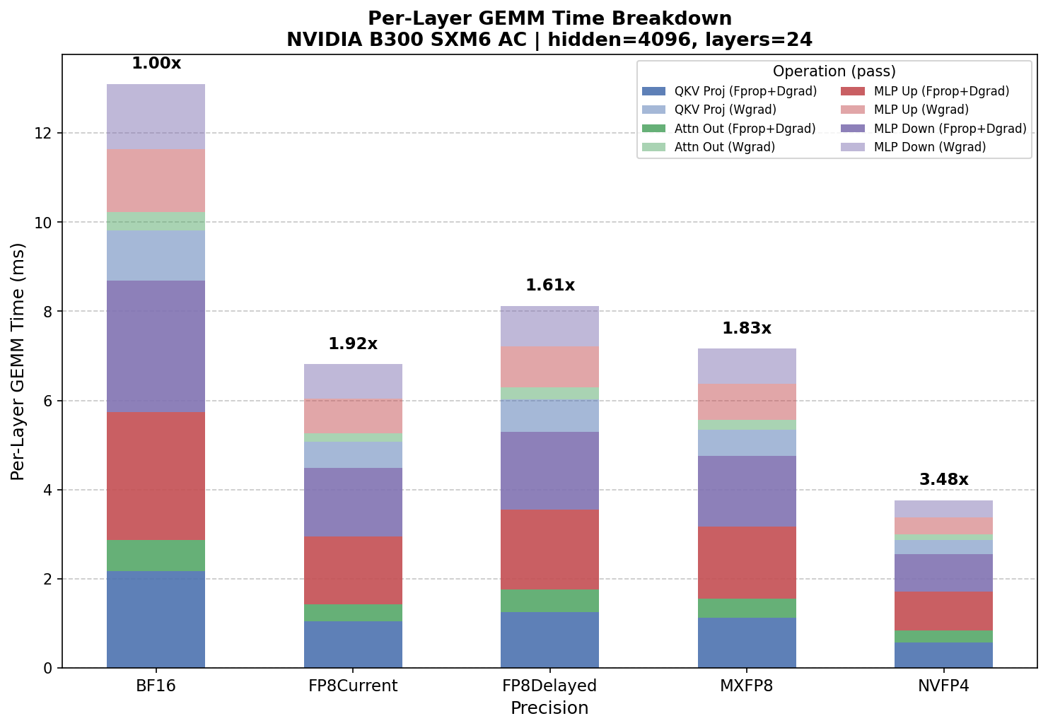
Pre-quantized model config benchmark – raw GEMM kernel throughput without quantization overhead.
Comparing the two tells you exactly how much quantization overhead costs: NVFP4 vs BF16 goes from 1.98x (autocast) to 3.48x (kernel-only). The gap between these two numbers is the overhead from dynamic quantization, Hadamard transforms, and block scaling that occurs in each training step.
Note
FP8 Block Scaling targets Hopper (SM90+), where it runs natively. On Blackwell (SM100+), FP8 Block is emulated via MXFP8 for backward compatibility – prefer MXFP8 or NVFP4 on Blackwell. See the Worked Example: 5B Model on H200 section below for Hopper-native FP8 Block Scaling benchmarks.
When to use which: Use autocast results for predicting real training speedups – that is what Transformer Engine actually does during training. Use pre-quantized results to understand whether quantization overhead is the bottleneck, or to compare raw tensor core throughput across precisions independent of the quantization implementation.
Worked Example: 5B Model on B300
Using a 5B-parameter model config (hidden=4096, intermediate=16384, MBS=31, seq_len=512, 24 layers), the full model config benchmark was run on a B300.
Looking at the per-shape NVFP4 vs MXFP8 speedups from the Fprop results:
QKV proj:   0.579 / 0.392  =  1.48x
Attn out:   0.269 / 0.256  =  1.05x  (barely faster -- overhead nearly matches GEMM gain)
MLP up:     0.924 / 0.635  =  1.46x
MLP down:   1.076 / 0.649  =  1.66x
A few things stand out:
The attn out GEMM (15872x4096x4096) gets minimal benefit from FP4. At 0.256 ms (NVFP4) vs 0.307 ms (BF16), the speedup is only 1.20x. This is the smallest weight matrix (4096x4096), and it is barely large enough for lower precision to overcome the overhead.
The big GEMMs show real but sub-theoretical gains. The FP4 tensor cores deliver 1.46–1.66x over MXFP8 on the large GEMMs – well short of the theoretical 2–3x from the hardware spec. Once you include the dead-weight attn out, the blended Fprop speedup drops to 1.47x. After adding Wgrad times, non-GEMM overhead (attention, layernorm, communication), and NVFP4-specific quantization costs (Hadamard transforms, stochastic rounding, 2D scaling), the end-to-end gap between NVFP4 and MXFP8 in training is consistent with these kernel-level numbers.
FP8 DelayedScaling is surprisingly competitive. At 7.80 ms/layer in autocast mode, it outperforms both FP8 CurrentScaling (9.15 ms) and MXFP8 (8.98 ms) on Blackwell. However, in pre-quantized mode FP8 CurrentScaling pulls ahead (6.81 ms vs 8.12 ms), suggesting DelayedScaling’s amax-history approach has lower quantization overhead but similar raw kernel throughput.
The pre-quantized results reveal the true kernel potential. Running with
--pre-quantize removes quantization overhead entirely, and NVFP4 vs BF16 jumps from
1.98x (autocast) to 3.48x (kernel-only). This shows the FP4 tensor cores are delivering
real speedup – it is the quantization overhead in autocast mode that narrows the gap.
The Fprop vs Dgrad comparison reveals that the x2 approximation is imprecise for quantized formats. While BF16 Dgrad is within 2% of Fprop, quantized formats show 5–13% slower Dgrad sums. The QKV Proj Dgrad is especially asymmetric – 33–51% slower than Fprop for FP8/FP4 – because swapping K (4096) and N (12288) dramatically changes the matrix aspect ratio and kernel selection.
Worked Example: 5B Model on H200
Using the same 5B-parameter model config on an NVIDIA H200 NVL (Hopper, SM90),
the available precision recipes are BF16, FP8 CurrentScaling, FP8 DelayedScaling,
and FP8 Block Scaling. MXFP8 and NVFP4 require Blackwell (SM100+/SM120+) and are
skipped with --no-fp8 --no-fp4.
GEMM Benchmark (Model Config Mode) on NVIDIA H200 NVL
Timing method: CUDA events
Mode: Autocast (includes quantization overhead)

==========================================================================================
Per-Layer GEMM Time:
                                  BF16 ms FP8Current ms FP8Delayed ms FP8Block ms
Fprop:                             10.653      6.503      6.188      7.425
Dgrad:                             10.813      6.795      6.306      7.636
Fprop + Dgrad:                     21.466     13.298     12.494     15.061
Wgrad:                             10.548      6.987      6.484      7.821
Per-layer total:                   32.014     20.285     18.978     22.882

Full Model (24 layers):
Total GEMM time (ms):             768.335    486.851    455.473    549.171

Estimated GEMM Speedups:
  FP8Delayed vs BF16:  1.69x
  FP8Current vs BF16:  1.58x
  FP8Block vs BF16:    1.40x
==========================================================================================
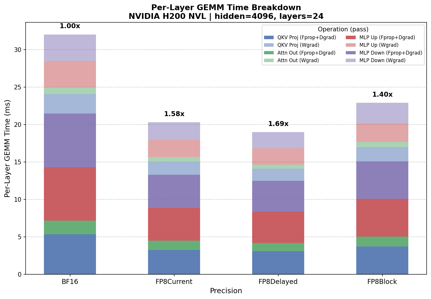
Autocast model config benchmark on NVIDIA H200 NVL – per-layer GEMM time breakdown by precision.
FP8 DelayedScaling is the fastest FP8 recipe on Hopper. At 18.98 ms/layer (1.69x over BF16), it outperforms both FP8 CurrentScaling (20.29 ms, 1.58x) and FP8 Block Scaling (22.88 ms, 1.40x). This is the same ordering seen on Blackwell, where DelayedScaling also outperforms CurrentScaling in autocast mode.
FP8 Block Scaling delivers the smallest speedup. At 1.40x over BF16, block scaling is slower than both tensor-wise FP8 approaches in autocast mode. The block scaling overhead – computing per-block scale factors for both rowwise and columnwise data – is not fully offset by the FP8 tensor core gains at these shapes.
In pre-quantized mode (raw kernel throughput), FP8 Block Scaling is excluded because the pre-quantized path produces 2D-by-2D block-scaled inputs, which Hopper’s cuBLAS does not support. Only FP8 CurrentScaling and FP8 DelayedScaling are benchmarked:
==========================================================================================
Per-Layer GEMM Time:
                                  BF16 ms FP8Current ms FP8Delayed ms
Fprop:                             10.632      5.577      6.207
Dgrad:                             10.747      5.661      6.375
Fprop + Dgrad:                     21.379     11.238     12.582
Wgrad:                             10.530      5.547      6.517
Per-layer total:                   31.968     16.785     19.099

Full Model (24 layers):
Total GEMM time (ms):             767.242    402.838    458.375

Estimated GEMM Speedups:
  FP8Current vs BF16:  1.90x
  FP8Delayed vs BF16:  1.67x
==========================================================================================
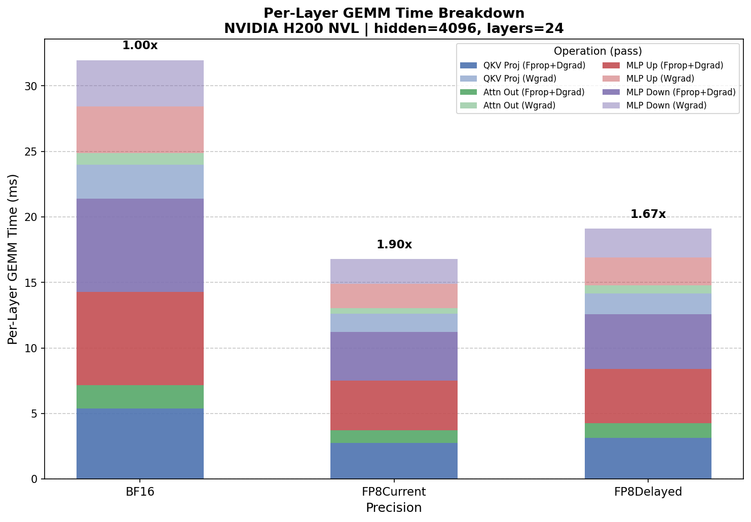
Pre-quantized model config benchmark on H200 – raw GEMM kernel throughput.
In pre-quantized mode, FP8 CurrentScaling pulls ahead. Without quantization
overhead, FP8 CurrentScaling reaches 1.90x over BF16, while FP8 DelayedScaling
shows 1.67x. FP8 DelayedScaling still runs in autocast mode even with
--pre-quantize (it relies on an amax history), so its pre-quantized times are
close to its autocast times (458 ms vs 455 ms). The gap between CurrentScaling’s
autocast (487 ms) and pre-quantized (403 ms) results reveals that ~17% of its
autocast time is quantization overhead.
Interpreting the Results
Once you have the GEMM-only speedup, compare it against your observed end-to-end training speedup:
GEMM speedup ~ training speedup – GEMMs are the bottleneck, everything is working as expected.
GEMM speedup >> training speedup – overhead outside of GEMMs is eating the gains. For NVFP4 in particular, this overhead includes Random Hadamard transforms on Wgrad inputs, stochastic rounding on gradients, 2D block scaling for weights, and the extra memory pass for per-tensor amax computation.
GEMM speedup ~ 1.0 even in the microbenchmark – the FP4 kernels are not actually faster at these shapes, or they are silently falling back to FP8.
The last case is especially worth checking. Set NVTE_LOG_LEVEL=1 or inspect with
Nsight Systems to confirm that Transformer Engine is actually dispatching FP4 kernels.
TE can silently fall back to FP8 or BF16 for layers or ops that do not support FP4
yet.
What GEMMs Do Not Cover
The linear projection GEMMs are the only ops where Transformer Engine’s precision setting (BF16 vs FP8 Block vs MXFP8 vs NVFP4) affects compute performance. The other major consumers in a transformer layer are precision-agnostic – they run the same regardless of which TE mode you use:
Attention (QK^T and softmax*V): Runs in BF16/FP16 via FlashAttention regardless of linear layer precision.
LayerNorm / RMSNorm: Typically in FP32, negligible cost.
Activation functions: Element-wise, memory-bound, unaffected by weight precision.
AllReduce (DDP/FSDP): Communication cost, independent of compute precision.
In addition, NVFP4 introduces precision-specific overhead that falls outside the GEMM kernels but is unique to FP4 mode. These ops do not exist in BF16 or MXFP8 and represent additional cost that NVFP4 must overcome to deliver a net speedup:
Random Hadamard transforms: 16x16 batched matmuls applied to both Wgrad inputs to improve quantization quality.
Stochastic rounding: Applied to gradients before FP4 quantization.
2D block scaling: Weight scaling with finer granularity than MXFP8’s 1D scaling.
Per-tensor amax passes: Extra memory pass to compute scaling factors.
This distinction matters: the precision-agnostic ops dilute GEMM speedups equally across all modes, but the NVFP4-specific ops actively widen the gap between NVFP4’s raw kernel speedup and its end-to-end speedup. This is why the autocast vs pre-quantized comparison is informative – the pre-quantized numbers show what the tensor cores can do, while the autocast numbers include both categories of overhead.
Manual Shape Mode
If you need to benchmark shapes that do not map to a standard transformer config –
diffusion models, mixture-of-experts, or non-standard architectures – or want to
profile individual GEMMs in isolation, you can pass explicit MxKxN triplets with the
--shapes flag:
# Fprop shapes for the 5B config
python benchmarks/gemm/benchmark_gemm.py -o roofline_fprop.png \
  --shapes 15872x4096x12288,15872x4096x4096,15872x4096x16384,15872x16384x4096

# Dgrad shapes (K and N swapped from Fprop)
python benchmarks/gemm/benchmark_gemm.py -o roofline_dgrad.png \
  --shapes 15872x12288x4096,15872x4096x4096,15872x16384x4096,15872x4096x16384

# Wgrad shapes
python benchmarks/gemm/benchmark_gemm.py -o roofline_wgrad.png \
  --shapes 4096x15872x12288,4096x15872x4096,4096x15872x16384,16384x15872x4096
This mode prints per-shape TFLOPS and ms but does not compute per-layer or full-model
totals – you would sum the ms values and compute speedups manually. The --shapes
flag is mutually exclusive with model config arguments.
Appendix: How the Shapes Are Derived
Note
This section is reference material – the tool handles all of this automatically. Read on if you want to understand the mechanics behind the shape derivation and speedup calculation.
The first thing to establish is M – the token dimension. Every linear layer in a
transformer operates on a 2D matrix of shape [tokens, features], where
tokens = micro_batch_size * sequence_length. For the example config:
M = 31 x 512 = 15,872
This is the batch dimension for every single GEMM in a forward or backward pass through one layer. It stays constant across all ops.
The Linear Layer Convention
Every linear layer computes Y = X @ W, which is a matrix multiply C = A x B
where:
A is the activation:
[M, K]B is the weight:
[K, N]C is the output:
[M, N]
The mapping is:
Symbol |
Meaning |
|---|---|
M |
Number of tokens ( |
K |
Input feature dimension (contracted/summed over) |
N |
Output feature dimension |
Your model config gives you K and N. Your batch config gives you M. That is all you need.
Note
Throughout this guide and in the tool’s output, GEMM shapes are written as
MxKxN – tokens x input features x output features. The --shapes flag
uses the same ordering.
Forward Pass GEMMs
A standard transformer layer has four major linear projections.
1. QKV Projection
Projects the input into queries, keys, and values as a single fused linear layer:
Input features (K) =
hidden_size= 4096Output features (N) = 3 x
hidden_size= 12,288
Y = X @ W_qkv
[15872, 4096] x [4096, 12288] -> [15872, 12288]

M = 15,872    K = 4,096    N = 12,288
2. Attention Output Projection
After attention, project back to the hidden dimension:
Input features (K) =
hidden_size= 4096Output features (N) =
hidden_size= 4096
Y = X @ W_out
[15872, 4096] x [4096, 4096] -> [15872, 4096]

M = 15,872    K = 4,096    N = 4,096
3. MLP Up Projection (Gate + Up)
The MLP first projects up to the intermediate dimension. In gated architectures (SwiGLU, etc.), this is typically fused into a single projection:
Input features (K) =
hidden_size= 4096Output features (N) =
intermediate_size= 16,384
Y = X @ W_up
[15872, 4096] x [4096, 16384] -> [15872, 16384]

M = 15,872    K = 4,096    N = 16,384
4. MLP Down Projection
Projects back from intermediate dimension to hidden dimension:
Input features (K) =
intermediate_size= 16,384Output features (N) =
hidden_size= 4096
Y = X @ W_down
[15872, 16384] x [16384, 4096] -> [15872, 4096]

M = 15,872    K = 16,384    N = 4,096
Forward Summary
Op |
Pass |
M |
K |
N |
Shape (MxKxN) |
FLOPs (2*M*K*N) |
|---|---|---|---|---|---|---|
QKV proj |
Forward |
15,872 |
4,096 |
12,288 |
15872x4096x12288 |
~1.60T |
Attn out proj |
Forward |
15,872 |
4,096 |
4,096 |
15872x4096x4096 |
~0.53T |
MLP up |
Forward |
15,872 |
4,096 |
16,384 |
15872x4096x16384 |
~2.13T |
MLP down |
Forward |
15,872 |
16,384 |
4,096 |
15872x16384x4096 |
~2.13T |
Total/layer |
~6.39T |
Backward Pass GEMMs
The backward pass through each linear layer produces two GEMMs: one for the gradient with respect to the input (dX), and one for the gradient with respect to the weights (dW).
Given forward Y = X @ W where X is [M, K] and W is [K, N]:
dX = dY @ W^T – The gradient flows back through the transposed weight matrix. The contraction axis is now N (the output features from the forward pass):
M = tokens K = out_features (N from forward) N = in_features (K from forward)
dW = X^T @ dY – The weight gradient contracts over the token dimension:
M = in_features K = tokens N = out_features
Full Backward Table
Op |
Pass |
M |
K |
N |
Shape (MxKxN) |
|---|---|---|---|---|---|
QKV proj |
Backward (dX) |
15,872 |
12,288 |
4,096 |
15872x12288x4096 |
QKV proj |
Backward (dW) |
4,096 |
15,872 |
12,288 |
4096x15872x12288 |
Attn out |
Backward (dX) |
15,872 |
4,096 |
4,096 |
15872x4096x4096 |
Attn out |
Backward (dW) |
4,096 |
15,872 |
4,096 |
4096x15872x4096 |
MLP up |
Backward (dX) |
15,872 |
16,384 |
4,096 |
15872x16384x4096 |
MLP up |
Backward (dW) |
4,096 |
15,872 |
16,384 |
4096x15872x16384 |
MLP down |
Backward (dX) |
15,872 |
4,096 |
16,384 |
15872x4096x16384 |
MLP down |
Backward (dW) |
16,384 |
15,872 |
4,096 |
16384x15872x4096 |
Total FLOP Budget
Each backward GEMM has the same FLOPs as its corresponding forward GEMM (the dimensions are just rearranged), and there are two per op, so:
Per layer: ~6.39T (fwd) + ~12.78T (bwd) = ~19.17 TFLOPS
Full model (24 layers): ~460 TFLOPS per step