Running Diagnostic Inference

Basic prognostic + diagnostic inference workflow.

This example will demonstrate how to run a deterministic inference workflow that couples a prognostic model with a diagnostic model. This diagnostic model will predict a new atmospheric quantity from the predicted fields of the prognostic.

In this example you will learn:

• How to instantiate a prognostic model
• How to instantiate a diagnostic model
• Creating a data source and IO object
• Running the built in diagnostic workflow
• Post-processing results

Set Up

All workflows inside Earth2Studio require constructed components to be handed to them. In this example, let's take a look at the diagnostic workflow: earth2studio.run.diagnostic.

Thus, we need the following:

• Prognostic Model: Use the built in FourCastNet Model earth2studio.models.px.FCN.
• Diagnostic Model: Use the built in precipitation AFNO model earth2studio.models.dx.PrecipitationAFNO.
• Datasource: Pull data from the GFS data api earth2studio.data.GFS.
• IO Backend: Save the outputs into a Zarr store earth2studio.io.ZarrBackend.

import os

os.makedirs("outputs", exist_ok=True)
from dotenv import load_dotenv

load_dotenv()  # TODO: make common example prep function

from earth2studio.data import GFS
from earth2studio.io import ZarrBackend
from earth2studio.models.dx import PrecipitationAFNO
from earth2studio.models.px import FCN
from earth2studio.utils.time import to_time_array

# Load the default model package which downloads the check point from NGC
package = FCN.load_default_package()
prognostic_model = FCN.load_model(package)

package = PrecipitationAFNO.load_default_package()
diagnostic_model = PrecipitationAFNO.load_model(package)

# Create the data source
data = GFS()

# Create the IO handler, store in memory
io = ZarrBackend()

Console output68 lines

Downloading config.json: 0%|          | 0.00/22.0 [00:00<?, ?B/s]
Downloading config.json: 100%|██████████| 22.0/22.0 [00:00<00:00, 121B/s]
Downloading config.json: 100%|██████████| 22.0/22.0 [00:00<00:00, 121B/s]

Downloading fcn.mdlus: 0%|          | 0.00/287M [00:00<?, ?B/s]
Downloading fcn.mdlus: 3%|▎         | 10.0M/287M [00:01<00:54, 5.29MB/s]
Downloading fcn.mdlus: 7%|▋         | 20.0M/287M [00:02<00:34, 8.12MB/s]
Downloading fcn.mdlus: 10%|█         | 30.0M/287M [00:03<00:29, 9.18MB/s]
Downloading fcn.mdlus: 14%|█▍        | 40.0M/287M [00:04<00:27, 9.34MB/s]
Downloading fcn.mdlus: 17%|█▋        | 50.0M/287M [00:06<00:27, 8.94MB/s]
Downloading fcn.mdlus: 21%|██        | 60.0M/287M [00:07<00:27, 8.56MB/s]
Downloading fcn.mdlus: 24%|██▍       | 70.0M/287M [00:08<00:27, 8.44MB/s]
Downloading fcn.mdlus: 28%|██▊       | 80.0M/287M [00:09<00:23, 9.24MB/s]
Downloading fcn.mdlus: 31%|███▏      | 90.0M/287M [00:10<00:20, 10.3MB/s]
Downloading fcn.mdlus: 35%|███▍      | 100M/287M [00:10<00:16, 11.7MB/s] 
Downloading fcn.mdlus: 38%|███▊      | 110M/287M [00:11<00:15, 12.0MB/s]
Downloading fcn.mdlus: 42%|████▏     | 120M/287M [00:12<00:13, 13.3MB/s]
Downloading fcn.mdlus: 45%|████▌     | 130M/287M [00:12<00:11, 14.4MB/s]
Downloading fcn.mdlus: 49%|████▊     | 140M/287M [00:13<00:09, 15.7MB/s]
Downloading fcn.mdlus: 52%|█████▏    | 150M/287M [00:14<00:08, 16.5MB/s]
Downloading fcn.mdlus: 56%|█████▌    | 160M/287M [00:14<00:07, 17.3MB/s]
Downloading fcn.mdlus: 59%|█████▉    | 170M/287M [00:15<00:06, 17.8MB/s]
Downloading fcn.mdlus: 63%|██████▎   | 180M/287M [00:15<00:06, 18.0MB/s]
Downloading fcn.mdlus: 66%|██████▌   | 190M/287M [00:16<00:05, 18.4MB/s]
Downloading fcn.mdlus: 70%|██████▉   | 200M/287M [00:16<00:05, 18.1MB/s]
Downloading fcn.mdlus: 73%|███████▎  | 210M/287M [00:17<00:04, 18.4MB/s]
Downloading fcn.mdlus: 77%|███████▋  | 220M/287M [00:18<00:03, 18.4MB/s]
Downloading fcn.mdlus: 80%|████████  | 230M/287M [00:18<00:03, 18.9MB/s]
Downloading fcn.mdlus: 84%|████████▎ | 240M/287M [00:19<00:02, 18.9MB/s]
Downloading fcn.mdlus: 87%|████████▋ | 250M/287M [00:19<00:02, 19.3MB/s]
Downloading fcn.mdlus: 91%|█████████ | 260M/287M [00:20<00:01, 20.2MB/s]
Downloading fcn.mdlus: 94%|█████████▍| 270M/287M [00:20<00:00, 20.3MB/s]
Downloading fcn.mdlus: 97%|█████████▋| 280M/287M [00:21<00:00, 21.0MB/s]
Downloading fcn.mdlus: 100%|██████████| 287M/287M [00:21<00:00, 20.8MB/s]
Downloading fcn.mdlus: 100%|██████████| 287M/287M [00:21<00:00, 14.1MB/s]

Downloading global_means.npy: 0%|          | 0.00/336 [00:00<?, ?B/s]
Downloading global_means.npy: 100%|██████████| 336/336 [00:00<00:00, 441B/s]
Downloading global_means.npy: 100%|██████████| 336/336 [00:00<00:00, 440B/s]

Downloading global_stds.npy: 0%|          | 0.00/336 [00:00<?, ?B/s]
Downloading global_stds.npy: 100%|██████████| 336/336 [00:01<00:00, 334B/s]
Downloading global_stds.npy: 100%|██████████| 336/336 [00:01<00:00, 333B/s]

Downloading precipitation_afno.zip: 0%|          | 0.00/261M [00:00<?, ?B/s]
Downloading precipitation_afno.zip: 0%|          | 1.26M/261M [00:00<00:20, 13.1MB/s]
Downloading precipitation_afno.zip: 3%|▎         | 7.24M/261M [00:00<00:06, 40.7MB/s]
Downloading precipitation_afno.zip: 7%|▋         | 17.2M/261M [00:00<00:03, 69.2MB/s]
Downloading precipitation_afno.zip: 12%|█▏        | 31.6M/261M [00:00<00:02, 101MB/s]
Downloading precipitation_afno.zip: 19%|█▊        | 48.7M/261M [00:00<00:01, 128MB/s]
Downloading precipitation_afno.zip: 25%|██▌       | 65.4M/261M [00:00<00:01, 143MB/s]
Downloading precipitation_afno.zip: 30%|███       | 79.1M/261M [00:00<00:01, 129MB/s]
Downloading precipitation_afno.zip: 35%|███▌      | 91.8M/261M [00:00<00:01, 122MB/s]
Downloading precipitation_afno.zip: 40%|███▉      | 104M/261M [00:01<00:01, 108MB/s] 
Downloading precipitation_afno.zip: 44%|████▍     | 116M/261M [00:01<00:01, 113MB/s]
Downloading precipitation_afno.zip: 49%|████▊     | 127M/261M [00:01<00:01, 110MB/s]
Downloading precipitation_afno.zip: 53%|█████▎    | 138M/261M [00:01<00:01, 89.9MB/s]
Downloading precipitation_afno.zip: 57%|█████▋    | 149M/261M [00:01<00:01, 95.2MB/s]
Downloading precipitation_afno.zip: 62%|██████▏   | 161M/261M [00:01<00:01, 99.1MB/s]
Downloading precipitation_afno.zip: 67%|██████▋   | 174M/261M [00:01<00:00, 107MB/s] 
Downloading precipitation_afno.zip: 71%|███████   | 185M/261M [00:01<00:00, 109MB/s]
Downloading precipitation_afno.zip: 75%|███████▌  | 196M/261M [00:01<00:00, 98.7MB/s]
Downloading precipitation_afno.zip: 80%|████████  | 209M/261M [00:02<00:00, 108MB/s] 
Downloading precipitation_afno.zip: 84%|████████▍ | 220M/261M [00:02<00:00, 106MB/s]
Downloading precipitation_afno.zip: 88%|████████▊ | 231M/261M [00:02<00:00, 104MB/s]
Downloading precipitation_afno.zip: 92%|█████████▏| 241M/261M [00:02<00:00, 101MB/s]
Downloading precipitation_afno.zip: 96%|█████████▌| 251M/261M [00:02<00:00, 88.2MB/s]
Downloading precipitation_afno.zip: 100%|██████████| 261M/261M [00:02<00:00, 103MB/s]

Fetch Data

You can easily fetch raw Xarray data from an initial condition data source with a simple call. By default, this caches the data locally on your machine, so you won't have to re-download it if you access it again or use it in an inference pipeline.

sample = data(
    to_time_array(["2024-01-01"]),
    prognostic_model.input_coords()["variable"],
)
print(sample)

Console output62 lines

Fetching GFS data:   0%|          | 0/26 [00:00<?, ?it/s]
Fetching GFS data:   4%|▍         | 1/26 [00:00<00:03,  6.36it/s]
Fetching GFS data:  23%|██▎       | 6/26 [00:00<00:02,  7.59it/s]
Fetching GFS data:  31%|███       | 8/26 [00:00<00:01,  9.14it/s]
Fetching GFS data:  50%|█████     | 13/26 [00:01<00:00, 15.56it/s]
Fetching GFS data:  62%|██████▏   | 16/26 [00:01<00:00, 10.74it/s]
Fetching GFS data:  69%|██████▉   | 18/26 [00:03<00:02,  3.28it/s]
Fetching GFS data:  77%|███████▋  | 20/26 [00:07<00:04,  1.30it/s]
Fetching GFS data:  81%|████████  | 21/26 [00:08<00:03,  1.47it/s]
Fetching GFS data:  88%|████████▊ | 23/26 [00:08<00:01,  1.75it/s]
Fetching GFS data:  92%|█████████▏| 24/26 [00:09<00:01,  1.75it/s]
Fetching GFS data:  96%|█████████▌| 25/26 [00:10<00:00,  1.52it/s]
Fetching GFS data: 100%|██████████| 26/26 [00:11<00:00,  1.43it/s]
Fetching GFS data: 100%|██████████| 26/26 [00:11<00:00,  2.34it/s]
<xarray.DataArray (time: 1, variable: 26, lat: 721, lon: 1440)> Size: 216MB
array([[[[-3.37807129e+00, -3.38807129e+00, -3.40807129e+00, ...,
          -3.33807129e+00, -3.34807129e+00, -3.36807129e+00],
         [-3.33807129e+00, -3.34807129e+00, -3.36807129e+00, ...,
          -3.28807129e+00, -3.30807129e+00, -3.31807129e+00],
         [-4.05807129e+00, -4.06807129e+00, -4.07807129e+00, ...,
          -3.99807129e+00, -4.01807129e+00, -4.03807129e+00],
         ...,
         [ 4.13192871e+00,  4.14192871e+00,  4.16192871e+00, ...,
           4.09192871e+00,  4.11192871e+00,  4.12192871e+00],
         [ 5.24192871e+00,  5.26192871e+00,  5.27192871e+00, ...,
           5.21192871e+00,  5.22192871e+00,  5.23192871e+00],
         [ 5.72192871e+00,  5.73192871e+00,  5.74192871e+00, ...,
           5.69192871e+00,  5.70192871e+00,  5.71192871e+00]],

        [[-3.13438721e+00, -3.11438721e+00, -3.10438721e+00, ...,
          -3.17438721e+00, -3.16438721e+00, -3.14438721e+00],
         [-3.23438721e+00, -3.21438721e+00, -3.20438721e+00, ...,
          -3.27438721e+00, -3.25438721e+00, -3.24438721e+00],
         [-3.72438721e+00, -3.70438721e+00, -3.69438721e+00, ...,
          -3.77438721e+00, -3.76438721e+00, -3.74438721e+00],
...
         [ 9.52740394e+04,  9.52732546e+04,  9.52728622e+04, ...,
           9.52760014e+04,  9.52752166e+04,  9.52748242e+04],
         [ 9.52579510e+04,  9.52571662e+04,  9.52567738e+04, ...,
           9.52587358e+04,  9.52583434e+04,  9.52579510e+04],
         [ 9.52442170e+04,  9.52442170e+04,  9.52442170e+04, ...,
           9.52442170e+04,  9.52442170e+04,  9.52442170e+04]],

        [[ 2.13206797e+02,  2.13206797e+02,  2.13206797e+02, ...,
           2.13206797e+02,  2.13206797e+02,  2.13206797e+02],
         [ 2.13416797e+02,  2.13416797e+02,  2.13406797e+02, ...,
           2.13416797e+02,  2.13416797e+02,  2.13416797e+02],
         [ 2.13756797e+02,  2.13756797e+02,  2.13746797e+02, ...,
           2.13766797e+02,  2.13766797e+02,  2.13766797e+02],
         ...,
         [ 2.13926797e+02,  2.13926797e+02,  2.13936797e+02, ...,
           2.13916797e+02,  2.13916797e+02,  2.13916797e+02],
         [ 2.13806797e+02,  2.13806797e+02,  2.13806797e+02, ...,
           2.13796797e+02,  2.13806797e+02,  2.13806797e+02],
         [ 2.13736797e+02,  2.13736797e+02,  2.13736797e+02, ...,
           2.13736797e+02,  2.13736797e+02,  2.13736797e+02]]]])
Coordinates:
  * time       (time) datetime64[ns] 8B 2024-01-01
  * variable   (variable) <U5 520B 'u10m' 'v10m' 't2m' ... 'v250' 'z250' 't250'
  * lat        (lat) float64 6kB 90.0 89.75 89.5 89.25 ... -89.5 -89.75 -90.0
  * lon        (lon) float64 12kB 0.0 0.25 0.5 0.75 ... 359.0 359.2 359.5 359.8
    lead_time  timedelta64[ns] 8B 00:00:00

Execute the Workflow

With all components initialized, running the workflow is a single line of Python code. Workflow will return the provided IO object back to the user, which can be used to then post process. Some have additional APIs that can be handy for post-processing or saving to file. Check the API docs for more information.

import earth2studio.run as run

nsteps = 8
io = run.diagnostic(
    ["2024-01-01"], nsteps, prognostic_model, diagnostic_model, data, io
)

print(io.root.tree())

Console output30 lines

2026-10-24 19:35:56.465 | INFO     | earth2studio.run:diagnostic:238 - Running diagnostic workflow!
2026-10-24 19:35:56.465 | INFO     | earth2studio.run:diagnostic:244 - Inference device: cuda

Fetching GFS data:   0%|          | 0/26 [00:00<?, ?it/s]
Fetching GFS data:   4%|▍         | 1/26 [00:00<00:19,  1.30it/s]
Fetching GFS data: 100%|██████████| 26/26 [00:00<00:00, 32.23it/s]
2026-10-24 19:35:57.566 | SUCCESS  | earth2studio.run:diagnostic:307 - Fetched data from GFS
2026-10-24 19:35:57.567 | INFO     | earth2studio.run:diagnostic:312 - Inference starting!


Running inference:   0%|          | 0/9 [00:00<?, ?it/s]

Running inference:  11%|█         | 1/9 [00:00<00:02,  3.75it/s]

Running inference:  33%|███▎      | 3/9 [00:00<00:00,  7.91it/s]

Running inference:  56%|█████▌    | 5/9 [00:00<00:00,  9.93it/s]

Running inference:  78%|███████▊  | 7/9 [00:00<00:00, 11.05it/s]

Running inference: 100%|██████████| 9/9 [00:00<00:00, 11.73it/s]
Running inference: 100%|██████████| 9/9 [00:00<00:00, 10.22it/s]
2026-10-24 19:35:58.449 | SUCCESS  | earth2studio.run:diagnostic:340 - 
Inference complete
/
├── lat (720,) float64
├── lead_time (9,) timedelta64[h]
├── lon (1440,) float64
├── time (1,) datetime64[ns]
└── tp (1, 9, 720, 1440) float32

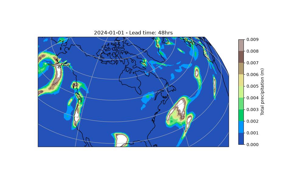
Post Processing

The last step is to plot the resulting predicted total precipitation. The power of diagnostic models is that they allow the prediction of any variable from a pre-trained prognostic model.

Note

The built in workflow will only save the direct outputs of the diagnostic. In this example only total precipitation is accessible for plotting. If you wish to save outputs of both the prognostic and diagnostic, we recommend writing a custom workflow.

from datetime import datetime

import cartopy.crs as ccrs
import matplotlib.pyplot as plt
import numpy as np

forecast = datetime(2024, 1, 1)
variable = "tp"
step = 8  # lead time = 48 hrs

plt.close("all")
# Create a Orthographic projection of USA
projection = ccrs.Orthographic(-100, 40)

# Create a figure and axes with the specified projection
fig, ax = plt.subplots(subplot_kw={"projection": projection}, figsize=(10, 6))

# Plot the field using pcolormesh
levels = np.arange(0.0, 0.01, 0.001)
im = ax.contourf(
    io["lon"][:],
    io["lat"][:],
    io[variable][0, step],
    levels,
    transform=ccrs.PlateCarree(),
    vmax=0.01,
    vmin=0.00,
    cmap="terrain",
)

# Set title
ax.set_title(f"{forecast.strftime('%Y-%m-%d')} - Lead time: {6*step}hrs")

# Add coastlines and gridlines6
ax.set_extent([220, 340, 20, 70])  # [lat min, lat max, lon min, lon max]
ax.coastlines()
ax.gridlines()
plt.colorbar(
    im, ax=ax, ticks=levels, shrink=0.75, pad=0.04, label="Total precipitation (m)"
)

plt.savefig("outputs/02_tp_prediction.jpg")

---

Download Python sourceDownload Jupyter notebookexecuted in 68.9s

Execution profile

Runtime telemetry

Profiled phases

Total runtime1m 9s

Setup56.8 s · 52 samples

Duration56.8 sTagged cells

CPU load5%Average · Peak 78%

Process memory2.1 GiBPeak resident set

Network received575.6 MiBHost-wide estimate

Network sent5.4 MiBHost-wide estimate

GPU utilization0%Peak 0%

GPU memory0.0 GiBof 79.6 GiB

GPU power69 WPeak draw

Inference2.3 s · 2 samples

Duration2.3 sTagged cells

CPU load8%Average · Peak 9%

Process memory2.5 GiBPeak resident set

Network received109.0 KiBHost-wide estimate

Network sent1.9 KiBHost-wide estimate

GPU utilization0%Peak 0%

GPU memory1.1 GiBof 79.6 GiB

GPU power76 WPeak draw

Plotting7.0 s · 7 samples

Duration7.0 sTagged cells

CPU load9%Average · Peak 10%

Process memory2.2 GiBPeak resident set

Network received1.8 KiBHost-wide estimate

Network sent1.7 KiBHost-wide estimate

GPU utilization13%Peak 91%

GPU memory2.6 GiBof 79.6 GiB

GPU power234 WPeak draw

Execution environment

CPUAMD EPYC 7313P 16-Core Processor

GPUNVIDIA H100 PCIe · 79.6 GiB

System RAM58.5 GiB

PlatformLinux 6.8.0-142-generic

Python3.13.13

GPU driver / CUDADriver 595.91.07 · CUDA support 13.2