Statistical Inference

Simple seasonal statistic inference workflow.

This example will demonstrate how to run a simple inference workflow to generate a forecast and then to save a statistic of that data. There are a handful of built-in statistics available in earth2studio.statistics, but here we will demonstrate how to define a custom statistic and run inference.

In this example you will learn:

• How to instantiate a built in prognostic model
• Creating a data source and IO object
• Create a custom statistic
• Running a simple built in workflow
• Post-processing results

Creating a Statistical Workflow

Start with creating a simple inference workflow to use. We encourage users to explore and experiment with their own custom workflows that borrow ideas from built in workflows inside earth2studio.run or the examples.

Creating our own generalizable workflow to use with statistics is easy when we rely on the component interfaces defined in Earth2Studio (use dependency injection). Here we create a run method that accepts the following:

• time: Input list of datetimes / strings to run inference for
• nsteps: Number of forecast steps to predict
• prognostic: Our initialized prognostic model
• statistic: our custom statistic
• data: Initialized data source to fetch initial conditions from
• io: IOBackend

We do not run an ensemble inference workflow here, even though it is common for statistical inference. See ensemble examples for details on how to extend this example for that purpose.

import os

os.makedirs("outputs", exist_ok=True)
from dotenv import load_dotenv

load_dotenv()  # TODO: make common example prep function

from datetime import datetime

import numpy as np
import pandas as pd
from loguru import logger
from tqdm import tqdm

from earth2studio.data import DataSource, fetch_data
from earth2studio.io import IOBackend
from earth2studio.models.px import PrognosticModel
from earth2studio.statistics import Statistic
from earth2studio.utils.coords import map_coords
from earth2studio.utils.time import to_time_array

logger.remove()
logger.add(lambda msg: tqdm.write(msg, end=""), colorize=True)


def run_stats(
    time: list[str] | list[datetime] | list[np.datetime64],
    nsteps: int,
    nensemble: int,
    prognostic: PrognosticModel,
    statistic: Statistic,
    data: DataSource,
    io: IOBackend,
) -> IOBackend:
    """Simple statistics workflow

    Parameters
    ----------
    time : list[str] | list[datetime] | list[np.datetime64]
        List of string, datetimes or np.datetime64
    nsteps : int
        Number of forecast steps
    nensemble : int
        Number of ensemble members to run inference for.
    prognostic : PrognosticModel
        Prognostic models
    statistic : Statistic
        Custom statistic to compute and write to IO.
    data : DataSource
        Data source
    io : IOBackend
        IO object

    Returns
    -------
    IOBackend
        Output IO object
    """
    logger.info("Running simple statistics workflow!")
    # Load model onto the device
    device = torch.device("cuda" if torch.cuda.is_available() else "cpu")
    logger.info(f"Inference device: {device}")
    prognostic = prognostic.to(device)
    # Fetch data from data source and load onto device
    time = to_time_array(time)
    x, coords = fetch_data(
        source=data,
        time=time,
        lead_time=prognostic.input_coords()["lead_time"],
        variable=prognostic.input_coords()["variable"],
        device=device,
    )
    logger.success(f"Fetched data from {data.__class__.__name__}")

    # Set up IO backend
    total_coords = coords.copy()
    output_coords = prognostic.output_coords(prognostic.input_coords())
    total_coords["lead_time"] = np.asarray(
        [output_coords["lead_time"] * i for i in range(nsteps + 1)]
    ).flatten()
    # Remove reduced dimensions from statistic
    for d in statistic.reduction_dimensions:
        total_coords.pop(d, None)

    io.add_array(total_coords, str(statistic))

    # Map lat and lon if needed
    x, coords = map_coords(x, coords, prognostic.input_coords())

    # Create prognostic iterator
    model = prognostic.create_iterator(x, coords)

    logger.info("Inference starting!")
    with tqdm(total=nsteps + 1, desc="Running inference") as pbar:
        for step, (x, coords) in enumerate(model):
            s, coords = statistic(x, coords)
            io.write(s, coords, str(statistic))
            pbar.update(1)
            if step == nsteps:
                break

    logger.success("Inference complete")
    return io

Console output9 lines

/__w/earth2studio/earth2studio/.venv/lib/python3.13/site-packages/torch/cuda/__init__.py:64: FutureWarning: The pynvml package is deprecated. Please install nvidia-ml-py instead. If you did not install pynvml directly, please report this to the maintainers of the package that installed pynvml for you.
  import pynvml  # type: ignore[import]
WARNING[XFORMERS]: xFormers can't load C++/CUDA extensions. xFormers was built for:
    PyTorch 2.10.0+cu128 with CUDA 1208 (you have 2.13.0+cu130)
    Python  3.10.19 (you have 3.13.13)
  Please reinstall xformers (see https://github.com/facebookresearch/xformers#installing-xformers)
  Memory-efficient attention, SwiGLU, sparse and more won't be available.
  Set XFORMERS_MORE_DETAILS=1 for more details
CuPy distance computation test failed with error: cuVS >= 24.12 or pylibraft < 24.12 should be installed to use this feature

Set Up

With the statistical workflow defined, we now need to create the individual components.

We need the following:

• Prognostic Model: Use the built in Pangu 24 hour model earth2studio.models.px.Pangu24.
• statistic: We define our own statistic: the Southern Oscillation Index (SOI).
• Datasource: Pull data from the GFS data api earth2studio.data.GFS.
• IO Backend: Save the outputs into a NetCDF4 store earth2studio.io.NetCDF4Backend.

from collections import OrderedDict

import fsspec
import numpy as np
import torch

from earth2studio.data import GFS
from earth2studio.io import NetCDF4Backend
from earth2studio.models.px import Pangu24
from earth2studio.utils.type import CoordSystem

# Load the default model package which downloads the check point from NGC
package = Pangu24.load_default_package()
model = Pangu24.load_model(package)

# Create the data source
data = GFS()

# Create the IO handler, store in memory
io = NetCDF4Backend(
    file_name="outputs/soi.nc",
    backend_kwargs={"mode": "w"},
)


# Create the custom statistic
class SOI:
    """Custom metric calculation the Southern Oscillation Index.

    SOI = ( standardized_tahiti_slp - standardized_darwin_slp ) / soi_normalization

    soi_normalization = std( historical ( standardized_tahiti_slp - standardized_darwin_slp ) )

    standardized_*_slp = (*_slp - climatological_mean_*_slp) / climatological_std_*_slp

    Note
    ----
    __str__
        Name that will be applied to the output of this statistic, primarily for IO purposes.
    reduction_dimensions
        Dimensions that this statistic reduces over. This is used to help automatically determine
        the output coordinates, primarily used for IO purposes.
    """

    def __str__(self) -> str:
        return "soi"

    def __init__(
        self,
    ):
        # Read in Tahiti and Darwin SLP data
        url = "https://data.longpaddock.qld.gov.au/SeasonalClimateOutlook/SouthernOscillationIndex/SOIDataFiles/DailySOI1933-1992Base.txt"
        with fsspec.open(url, "r") as f:
            ds = pd.read_csv(f, sep=r"\s+")
        dates = pd.date_range("1999-01-01", freq="d", periods=len(ds))
        ds["date"] = dates
        ds = ds.set_index("date")
        ds = ds.drop(["Year", "Day", "SOI"], axis=1)
        ds = ds.rolling(30, min_periods=1).mean().dropna()

        self.climatological_means = torch.tensor(
            ds.groupby(ds.index.month).mean().to_numpy(), dtype=torch.float32
        )
        self.climatological_std = torch.tensor(
            ds.groupby(ds.index.month).std().to_numpy(), dtype=torch.float32
        )

        standardized = ds.groupby(ds.index.month).transform(
            lambda x: (x - x.mean()) / x.std()
        )
        diff = standardized["Tahiti"] - standardized["Darwin"]

        self.normalization = torch.tensor(
            diff.groupby(ds.index.month).std().to_numpy(), dtype=torch.float32
        )

        self.tahiti_coords = {
            "variable": np.array(["msl"]),
            "lat": np.array([-17.65]),
            "lon": np.array([210.57]),
        }
        self.darwin_coords = {
            "variable": np.array(["msl"]),
            "lat": np.array([-12.46]),
            "lon": np.array([130.84]),
        }

        self.reduction_dimensions = list(self.tahiti_coords)

    def __call__(
        self, x: torch.Tensor, coords: CoordSystem
    ) -> tuple[torch.Tensor, CoordSystem]:
        """Computes the SOI given an input.

        coords must be a superset of both

        tahiti_coords = {
            'variable': np.array(['msl']),
            'lat': np.array([-17.65]),
            'lon': np.array([210.57])
        }

        and

        darwin_coords = {
            'variable': np.array(['msl']),
            'lat': np.array([-12.46]),
            'lon': np.array([130.84])
        }

        So make sure that the model chosen predicts the `msl` variable.

        Parameters
        ----------
        x : torch.Tensor
            Input tensor
        coords : CoordSystem
            coordinate system belonging to the input tensor.

        Returns
        -------
        tuple[torch.Tensor, CoordSystem]
            Returns the SOI and appropriate coordinate system.
        """
        tahiti, _ = map_coords(x, coords, self.tahiti_coords)
        darwin, _ = map_coords(x, coords, self.darwin_coords)

        tahiti = tahiti.squeeze(-3, -2, -1) / 100.0
        darwin = darwin.squeeze(-3, -2, -1) / 100.0
        output_coords = OrderedDict(
            {k: v for k, v in coords.items() if k not in self.reduction_dimensions}
        )

        # Get time coordinates
        times = coords["time"].reshape(-1, 1) + coords["lead_time"].reshape(1, -1)
        months = torch.broadcast_to(
            torch.as_tensor(
                [pd.Timestamp(t).month for t in times.flatten()],
                device=tahiti.device,
                dtype=torch.int32,
            ).reshape(times.shape),
            tahiti.shape,
        )

        cm = self.climatological_means.to(tahiti.device)
        cs = self.climatological_std.to(tahiti.device)
        norm = self.normalization.to(tahiti.device)

        tahiti_std_anomaly = (tahiti - cm[months, 0]) / cs[months, 0]
        darwin_std_anomaly = (tahiti - cm[months, 1]) / cs[months, 1]

        return (tahiti_std_anomaly - darwin_std_anomaly) / norm[months], output_coords


soi = SOI()

Console output66 lines

Downloading pangu_weather_24.onnx: 0%|          | 0.00/1.10G [00:00<?, ?B/s]
Downloading pangu_weather_24.onnx: 1%|          | 10.0M/1.10G [00:01<02:01, 9.64MB/s]
Downloading pangu_weather_24.onnx: 2%|▏         | 20.0M/1.10G [00:01<00:56, 20.6MB/s]
Downloading pangu_weather_24.onnx: 3%|▎         | 30.0M/1.10G [00:01<00:35, 32.2MB/s]
Downloading pangu_weather_24.onnx: 4%|▍         | 50.0M/1.10G [00:01<00:21, 53.2MB/s]
Downloading pangu_weather_24.onnx: 5%|▌         | 60.0M/1.10G [00:01<00:18, 61.3MB/s]
Downloading pangu_weather_24.onnx: 6%|▌         | 70.0M/1.10G [00:02<00:45, 24.2MB/s]
Downloading pangu_weather_24.onnx: 7%|▋         | 80.0M/1.10G [00:02<00:35, 30.7MB/s]
Downloading pangu_weather_24.onnx: 8%|▊         | 90.0M/1.10G [00:02<00:28, 38.8MB/s]
Downloading pangu_weather_24.onnx: 10%|▉         | 110M/1.10G [00:03<00:19, 54.5MB/s]
Downloading pangu_weather_24.onnx: 11%|█         | 120M/1.10G [00:03<00:17, 61.6MB/s]
Downloading pangu_weather_24.onnx: 12%|█▏        | 140M/1.10G [00:03<00:13, 73.9MB/s]
Downloading pangu_weather_24.onnx: 13%|█▎        | 150M/1.10G [00:03<00:12, 79.1MB/s]
Downloading pangu_weather_24.onnx: 14%|█▍        | 160M/1.10G [00:03<00:12, 82.7MB/s]
Downloading pangu_weather_24.onnx: 16%|█▌        | 180M/1.10G [00:03<00:10, 90.4MB/s]
Downloading pangu_weather_24.onnx: 18%|█▊        | 200M/1.10G [00:04<00:10, 95.3MB/s]
Downloading pangu_weather_24.onnx: 20%|█▉        | 220M/1.10G [00:04<00:09, 101MB/s] 
Downloading pangu_weather_24.onnx: 21%|██▏       | 240M/1.10G [00:04<00:09, 103MB/s]
Downloading pangu_weather_24.onnx: 23%|██▎       | 260M/1.10G [00:04<00:08, 103MB/s]
Downloading pangu_weather_24.onnx: 25%|██▍       | 280M/1.10G [00:04<00:08, 104MB/s]
Downloading pangu_weather_24.onnx: 27%|██▋       | 300M/1.10G [00:04<00:08, 106MB/s]
Downloading pangu_weather_24.onnx: 28%|██▊       | 320M/1.10G [00:05<00:07, 110MB/s]
Downloading pangu_weather_24.onnx: 30%|███       | 340M/1.10G [00:05<00:07, 110MB/s]
Downloading pangu_weather_24.onnx: 32%|███▏      | 360M/1.10G [00:05<00:07, 108MB/s]
Downloading pangu_weather_24.onnx: 34%|███▎      | 380M/1.10G [00:05<00:07, 107MB/s]
Downloading pangu_weather_24.onnx: 35%|███▌      | 400M/1.10G [00:05<00:07, 107MB/s]
Downloading pangu_weather_24.onnx: 37%|███▋      | 420M/1.10G [00:06<00:06, 110MB/s]
Downloading pangu_weather_24.onnx: 39%|███▉      | 440M/1.10G [00:06<00:06, 112MB/s]
Downloading pangu_weather_24.onnx: 41%|████      | 460M/1.10G [00:06<00:06, 106MB/s]
Downloading pangu_weather_24.onnx: 43%|████▎     | 480M/1.10G [00:06<00:06, 105MB/s]
Downloading pangu_weather_24.onnx: 44%|████▍     | 500M/1.10G [00:06<00:06, 106MB/s]
Downloading pangu_weather_24.onnx: 46%|████▌     | 520M/1.10G [00:07<00:05, 109MB/s]
Downloading pangu_weather_24.onnx: 48%|████▊     | 540M/1.10G [00:07<00:05, 107MB/s]
Downloading pangu_weather_24.onnx: 50%|████▉     | 560M/1.10G [00:07<00:05, 108MB/s]
Downloading pangu_weather_24.onnx: 51%|█████▏    | 580M/1.10G [00:07<00:05, 109MB/s]
Downloading pangu_weather_24.onnx: 53%|█████▎    | 600M/1.10G [00:07<00:05, 110MB/s]
Downloading pangu_weather_24.onnx: 55%|█████▌    | 620M/1.10G [00:08<00:04, 108MB/s]
Downloading pangu_weather_24.onnx: 57%|█████▋    | 640M/1.10G [00:08<00:04, 106MB/s]
Downloading pangu_weather_24.onnx: 59%|█████▊    | 660M/1.10G [00:08<00:04, 107MB/s]
Downloading pangu_weather_24.onnx: 60%|██████    | 680M/1.10G [00:08<00:04, 109MB/s]
Downloading pangu_weather_24.onnx: 62%|██████▏   | 700M/1.10G [00:08<00:04, 112MB/s]
Downloading pangu_weather_24.onnx: 64%|██████▍   | 720M/1.10G [00:09<00:03, 112MB/s]
Downloading pangu_weather_24.onnx: 66%|██████▌   | 740M/1.10G [00:09<00:03, 108MB/s]
Downloading pangu_weather_24.onnx: 67%|██████▋   | 760M/1.10G [00:09<00:03, 107MB/s]
Downloading pangu_weather_24.onnx: 69%|██████▉   | 780M/1.10G [00:09<00:03, 106MB/s]
Downloading pangu_weather_24.onnx: 71%|███████   | 800M/1.10G [00:09<00:03, 106MB/s]
Downloading pangu_weather_24.onnx: 73%|███████▎  | 820M/1.10G [00:10<00:03, 106MB/s]
Downloading pangu_weather_24.onnx: 75%|███████▍  | 840M/1.10G [00:10<00:02, 107MB/s]
Downloading pangu_weather_24.onnx: 76%|███████▋  | 860M/1.10G [00:10<00:02, 109MB/s]
Downloading pangu_weather_24.onnx: 78%|███████▊  | 880M/1.10G [00:10<00:02, 110MB/s]
Downloading pangu_weather_24.onnx: 80%|███████▉  | 900M/1.10G [00:10<00:02, 111MB/s]
Downloading pangu_weather_24.onnx: 82%|████████▏ | 920M/1.10G [00:10<00:01, 109MB/s]
Downloading pangu_weather_24.onnx: 83%|████████▎ | 940M/1.10G [00:11<00:01, 108MB/s]
Downloading pangu_weather_24.onnx: 85%|████████▌ | 960M/1.10G [00:11<00:01, 106MB/s]
Downloading pangu_weather_24.onnx: 87%|████████▋ | 980M/1.10G [00:11<00:01, 103MB/s]
Downloading pangu_weather_24.onnx: 88%|████████▊ | 990M/1.10G [00:11<00:01, 103MB/s]
Downloading pangu_weather_24.onnx: 89%|████████▊ | 0.98G/1.10G [00:11<00:01, 100MB/s]
Downloading pangu_weather_24.onnx: 90%|████████▉ | 0.99G/1.10G [00:11<00:01, 97.9MB/s]
Downloading pangu_weather_24.onnx: 91%|█████████▏| 1.01G/1.10G [00:12<00:01, 101MB/s] 
Downloading pangu_weather_24.onnx: 92%|█████████▏| 1.02G/1.10G [00:12<00:00, 101MB/s]
Downloading pangu_weather_24.onnx: 94%|█████████▍| 1.04G/1.10G [00:12<00:00, 99.4MB/s]
Downloading pangu_weather_24.onnx: 96%|█████████▌| 1.05G/1.10G [00:12<00:00, 102MB/s] 
Downloading pangu_weather_24.onnx: 98%|█████████▊| 1.07G/1.10G [00:12<00:00, 104MB/s]
Downloading pangu_weather_24.onnx: 98%|█████████▊| 1.08G/1.10G [00:12<00:00, 103MB/s]
Downloading pangu_weather_24.onnx: 100%|██████████| 1.10G/1.10G [00:13<00:00, 105MB/s]
Downloading pangu_weather_24.onnx: 100%|██████████| 1.10G/1.10G [00:13<00:00, 90.1MB/s]

Execute the Workflow

With all components initialized, running the workflow is a single line of Python code. Workflow will return the provided IO object back to the user, which can be used to then post process. Some have additional APIs that can be handy for post-processing or saving to file. Check the API docs for more information. We simulate a trajectory of 60 time steps, or 2 months using Pangu24

nsteps = 60
nensemble = 1
io = run_stats(["2022-01-01"], nsteps, nensemble, model, soi, data, io)

Console output82 lines

2026-08-15 05:54:22.102 | INFO     | __main__:run_stats:59 - Running simple statistics workflow!
2026-08-15 05:54:22.102 | INFO     | __main__:run_stats:62 - Inference device: cuda

Fetching GFS data:   0%|          | 0/69 [00:00<?, ?it/s]
Fetching GFS data:   1%|▏         | 1/69 [00:00<00:30,  2.21it/s]
Fetching GFS data:   3%|▎         | 2/69 [00:00<00:18,  3.59it/s]
Fetching GFS data:   9%|▊         | 6/69 [00:00<00:05, 11.12it/s]
Fetching GFS data:  12%|█▏        | 8/69 [00:00<00:04, 13.09it/s]
Fetching GFS data:  14%|█▍        | 10/69 [00:01<00:04, 12.92it/s]
Fetching GFS data:  17%|█▋        | 12/69 [00:01<00:04, 12.87it/s]
Fetching GFS data:  29%|██▉       | 20/69 [00:01<00:03, 13.97it/s]
Fetching GFS data:  32%|███▏      | 22/69 [00:01<00:03, 14.55it/s]
Fetching GFS data:  59%|█████▉    | 41/69 [00:02<00:00, 33.47it/s]
Fetching GFS data:  81%|████████  | 56/69 [00:02<00:00, 50.74it/s]
Fetching GFS data:  94%|█████████▍| 65/69 [00:02<00:00, 53.68it/s]
Fetching GFS data: 100%|██████████| 69/69 [00:02<00:00, 29.33it/s]
2026-08-15 05:54:38.302 | SUCCESS  | __main__:run_stats:73 - Fetched data from GFS
2026-08-15 05:54:38.305 | INFO     | __main__:run_stats:93 - Inference starting!

Running inference:   0%|          | 0/61 [00:00<?, ?it/s]
Running inference:   3%|▎         | 2/61 [00:01<00:32,  1.80it/s]
Running inference:   5%|▍         | 3/61 [00:01<00:33,  1.74it/s]
Running inference:   7%|▋         | 4/61 [00:02<00:33,  1.71it/s]
Running inference:   8%|▊         | 5/61 [00:02<00:33,  1.69it/s]
Running inference:  10%|▉         | 6/61 [00:03<00:32,  1.68it/s]
Running inference:  11%|█▏        | 7/61 [00:04<00:32,  1.67it/s]
Running inference:  13%|█▎        | 8/61 [00:04<00:31,  1.67it/s]
Running inference:  15%|█▍        | 9/61 [00:05<00:31,  1.66it/s]
Running inference:  16%|█▋        | 10/61 [00:05<00:30,  1.66it/s]
Running inference:  18%|█▊        | 11/61 [00:06<00:30,  1.66it/s]
Running inference:  20%|█▉        | 12/61 [00:07<00:29,  1.66it/s]
Running inference:  21%|██▏       | 13/61 [00:07<00:28,  1.66it/s]
Running inference:  23%|██▎       | 14/61 [00:08<00:28,  1.66it/s]
Running inference:  25%|██▍       | 15/61 [00:08<00:27,  1.66it/s]
Running inference:  26%|██▌       | 16/61 [00:09<00:27,  1.66it/s]
Running inference:  28%|██▊       | 17/61 [00:10<00:26,  1.66it/s]
Running inference:  30%|██▉       | 18/61 [00:10<00:25,  1.66it/s]
Running inference:  31%|███       | 19/61 [00:11<00:25,  1.66it/s]
Running inference:  33%|███▎      | 20/61 [00:11<00:24,  1.66it/s]
Running inference:  34%|███▍      | 21/61 [00:12<00:24,  1.66it/s]
Running inference:  36%|███▌      | 22/61 [00:13<00:23,  1.66it/s]
Running inference:  38%|███▊      | 23/61 [00:13<00:22,  1.66it/s]
Running inference:  39%|███▉      | 24/61 [00:14<00:22,  1.66it/s]
Running inference:  41%|████      | 25/61 [00:14<00:21,  1.66it/s]
Running inference:  43%|████▎     | 26/61 [00:15<00:21,  1.66it/s]
Running inference:  44%|████▍     | 27/61 [00:16<00:20,  1.66it/s]
Running inference:  46%|████▌     | 28/61 [00:16<00:19,  1.66it/s]
Running inference:  48%|████▊     | 29/61 [00:17<00:19,  1.66it/s]
Running inference:  49%|████▉     | 30/61 [00:17<00:18,  1.66it/s]
Running inference:  51%|█████     | 31/61 [00:18<00:18,  1.66it/s]
Running inference:  52%|█████▏    | 32/61 [00:19<00:17,  1.66it/s]
Running inference:  54%|█████▍    | 33/61 [00:19<00:16,  1.66it/s]
Running inference:  56%|█████▌    | 34/61 [00:20<00:16,  1.66it/s]
Running inference:  57%|█████▋    | 35/61 [00:21<00:15,  1.66it/s]
Running inference:  59%|█████▉    | 36/61 [00:21<00:15,  1.66it/s]
Running inference:  61%|██████    | 37/61 [00:22<00:14,  1.66it/s]
Running inference:  62%|██████▏   | 38/61 [00:22<00:13,  1.66it/s]
Running inference:  64%|██████▍   | 39/61 [00:23<00:13,  1.66it/s]
Running inference:  66%|██████▌   | 40/61 [00:24<00:12,  1.66it/s]
Running inference:  67%|██████▋   | 41/61 [00:24<00:12,  1.66it/s]
Running inference:  69%|██████▉   | 42/61 [00:25<00:11,  1.66it/s]
Running inference:  70%|███████   | 43/61 [00:25<00:10,  1.66it/s]
Running inference:  72%|███████▏  | 44/61 [00:26<00:10,  1.66it/s]
Running inference:  74%|███████▍  | 45/61 [00:27<00:09,  1.66it/s]
Running inference:  75%|███████▌  | 46/61 [00:27<00:09,  1.65it/s]
Running inference:  77%|███████▋  | 47/61 [00:28<00:08,  1.65it/s]
Running inference:  79%|███████▊  | 48/61 [00:28<00:07,  1.66it/s]
Running inference:  80%|████████  | 49/61 [00:29<00:07,  1.66it/s]
Running inference:  82%|████████▏ | 50/61 [00:30<00:06,  1.65it/s]
Running inference:  84%|████████▎ | 51/61 [00:30<00:06,  1.65it/s]
Running inference:  85%|████████▌ | 52/61 [00:31<00:05,  1.65it/s]
Running inference:  87%|████████▋ | 53/61 [00:31<00:04,  1.65it/s]
Running inference:  89%|████████▊ | 54/61 [00:32<00:04,  1.65it/s]
Running inference:  90%|█████████ | 55/61 [00:33<00:03,  1.65it/s]
Running inference:  92%|█████████▏| 56/61 [00:33<00:03,  1.65it/s]
Running inference:  93%|█████████▎| 57/61 [00:34<00:02,  1.65it/s]
Running inference:  95%|█████████▌| 58/61 [00:34<00:01,  1.65it/s]
Running inference:  97%|█████████▋| 59/61 [00:35<00:01,  1.65it/s]
Running inference:  98%|█████████▊| 60/61 [00:36<00:00,  1.65it/s]
Running inference: 100%|██████████| 61/61 [00:36<00:00,  1.65it/s]
Running inference: 100%|██████████| 61/61 [00:36<00:00,  1.66it/s]
2026-08-15 05:55:15.040 | SUCCESS  | __main__:run_stats:102 - Inference complete

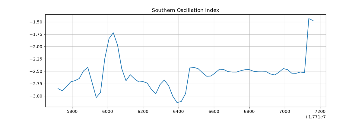
Post Processing

The last step is to post process our results.

Notice that the NetCDF IO function has additional APIs to interact with the stored data.

import matplotlib.pyplot as plt

times = io["time"][:].flatten() + io["lead_time"][:].flatten()

fig = plt.figure(figsize=(12, 4))
ax = fig.add_subplot(1, 1, 1)
ax.plot(times, io["soi"][:].flatten())
ax.set_title("Southern Oscillation Index")
ax.grid("on")

plt.savefig("outputs/07_southern_oscillation_index_prediction_2022.png")
io.close()

---

Download Python sourceDownload Jupyter notebookexecuted in 110.0s

Execution profile

Runtime telemetry

Total runtime1m 50s

Execution environment

CPUAMD EPYC 7313P 16-Core Processor

GPUNVIDIA H100 PCIe · 79.6 GiB

System RAM58.5 GiB

PlatformLinux 6.8.0-136-generic

Python3.13.13

GPU driver / CUDADriver 595.84 · CUDA support 13.2