Running DLESyM Inference
Basic deterministic inference workflow for the DLESyM model.
This example will demonstrate how to run a simple inference workflow with the DLESyM model, which differs from other prognostic models in earth2studio. DLESyM performs global earth system modeling, including atmosphere and ocean components which evolve on different timescales (different temporal resolution). Internally, the model uses a HEALPix nside=64 (approximately 1 degree) resolution grid for the physical variables of interest. The model also uses some derived input variables which are not provided by standard data sources but can be computed from the standard variables.
In this example you will learn:
- How to instantiate the DLESyM model
- How to use the model API to generate a forecast
- How to use the output selection and regridding methods to select appropriate data
- How to use the DLESyMLatLon model with earth2studio workflows
Set Up
The first step is fetching appropriate input data for the model. The ERA5 data sources in earth2studio provide data on the lat/lon grid, so have two options:
- Use the
earth2studio.models.px.DLESyMLatLonmodel. This version of DLESyM accepts inputs on the lat/lon grid and regrids them to the HEALPix grid internally, before returning the output regridded back to the lat/lon grid. This is the recommended approach for most users as it can be used directly with earth2studio data sources and workflows, since it performs regridding and pre-processing internally. - Use the
earth2studio.models.px.DLESyMmodel, and handle the regridding of input lat/lon data ourselves. Since the model uses some derived variables which are not provided by the data source, we would also need to prepare these derived variables ourselves.
Let's load both of these models and inspect the expected input coordinates for each. Also note the input and output variable set for each model.
import os

os.makedirs("outputs", exist_ok=True)
from dotenv import load_dotenv

load_dotenv()  # TODO: make common example prep function
import numpy as np
import torch

from earth2studio.data import ARCO_ERA5
from earth2studio.data.utils import fetch_data
from earth2studio.models.px.dlesym import DLESyM, DLESyMLatLon

device = "cuda"
if not torch.cuda.is_available():
    raise RuntimeError("GPU/CUDA required for DLESyM")

# Create the data source
data = ARCO_ERA5()


# Load the default model package
package = DLESyMLatLon.load_default_package()
model_ll = DLESyMLatLon.load_model(package).to(device)
package = DLESyM.load_default_package()
model_hpx = DLESyM.load_model(package).to(device)

in_coords_ll = model_ll.input_coords()
in_coords_hpx = model_hpx.input_coords()
print(
    "DLESyM LatLon input coord shapes: ",
    [(k, v.shape) for k, v in in_coords_ll.items()],
)
print(
    "DLESyM HPX input coord shapes: ", [(k, v.shape) for k, v in in_coords_hpx.items()]
)
print("Lat-lon input variable names: ", in_coords_ll["variable"])
print(
    "Lat-lon output variable names: ", model_ll.output_coords(in_coords_ll)["variable"]
)
print("HEALPix input variable names: ", in_coords_hpx["variable"])
print(
    "HEALPix output variable names: ",
    model_hpx.output_coords(in_coords_hpx)["variable"],
)
Console output43 lines
Downloading config.yaml: 0%|          | 0.00/955 [00:00<?, ?B/s]
Downloading config.yaml: 100%|██████████| 955/955 [00:00<00:00, 3.96kB/s]
Downloading config.yaml: 100%|██████████| 955/955 [00:00<00:00, 3.94kB/s]

Downloading config.yaml: 0%|          | 0.00/1.50k [00:00<?, ?B/s]
Downloading config.yaml: 100%|██████████| 1.50k/1.50k [00:00<00:00, 5.89kB/s]
Downloading config.yaml: 100%|██████████| 1.50k/1.50k [00:00<00:00, 5.87kB/s]

Downloading atmos_model_0.mdlus: 0%|          | 0.00/19.7M [00:00<?, ?B/s]
Downloading atmos_model_0.mdlus: 51%|█████     | 10.0M/19.7M [00:01<00:01, 7.20MB/s]
Downloading atmos_model_0.mdlus: 100%|██████████| 19.7M/19.7M [00:01<00:00, 15.5MB/s]
Downloading atmos_model_0.mdlus: 100%|██████████| 19.7M/19.7M [00:01<00:00, 13.1MB/s]

Downloading ocean_model_0.mdlus: 0%|          | 0.00/18.6M [00:00<?, ?B/s]
Downloading ocean_model_0.mdlus: 54%|█████▎    | 10.0M/18.6M [00:01<00:01, 7.99MB/s]
Downloading ocean_model_0.mdlus: 100%|██████████| 18.6M/18.6M [00:01<00:00, 15.4MB/s]
Downloading ocean_model_0.mdlus: 100%|██████████| 18.6M/18.6M [00:01<00:00, 13.2MB/s]

Downloading hpx_lat.npy: 0%|          | 0.00/384k [00:00<?, ?B/s]
Downloading hpx_lat.npy: 100%|██████████| 384k/384k [00:00<00:00, 446kB/s]
Downloading hpx_lat.npy: 100%|██████████| 384k/384k [00:00<00:00, 446kB/s]

Downloading hpx_lon.npy: 0%|          | 0.00/384k [00:00<?, ?B/s]
Downloading hpx_lon.npy: 100%|██████████| 384k/384k [00:00<00:00, 711kB/s]
Downloading hpx_lon.npy: 100%|██████████| 384k/384k [00:00<00:00, 708kB/s]

Downloading land_sea_mask.npy: 0%|          | 0.00/192k [00:00<?, ?B/s]
Downloading land_sea_mask.npy: 100%|██████████| 192k/192k [00:00<00:00, 304kB/s]
Downloading land_sea_mask.npy: 100%|██████████| 192k/192k [00:00<00:00, 303kB/s]

Downloading topography.npy: 0%|          | 0.00/192k [00:00<?, ?B/s]
Downloading topography.npy: 100%|██████████| 192k/192k [00:00<00:00, 264kB/s]
Downloading topography.npy: 100%|██████████| 192k/192k [00:00<00:00, 263kB/s]
DLESyM LatLon input coord shapes:  [('batch', (0,)), ('time', (0,)), ('lead_time', (9,)), ('variable', (12,)), ('lat', (721,)), ('lon', (1440,))]
DLESyM HPX input coord shapes:  [('batch', (0,)), ('time', (0,)), ('lead_time', (9,)), ('variable', (10,)), ('face', (12,)), ('height', (64,)), ('width', (64,))]
Lat-lon input variable names:  ['z500' 'z1000' 't2m' 'tcwv' 't850' 'z250' 'ttr03' 'sst' 'u10m' 'v10m'
 'z300' 'z700']
Lat-lon output variable names:  ['z500' 'tau300-700' 'z1000' 't2m' 'tcwv' 't850' 'z250' 'ws10m' 'ttr03'
 'tp6' 'msl' 'sst']
HEALPix input variable names:  ['z500' 'tau300-700' 'z1000' 't2m' 'tcwv' 't850' 'z250' 'ws10m' 'ttr03'
 'sst']
HEALPix output variable names:  ['z500' 'tau300-700' 'z1000' 't2m' 'tcwv' 't850' 'z250' 'ws10m' 'ttr03'
 'tp6' 'msl' 'sst']
Making Predictions, Regridding, and Selecting Outputs
Let's now pull some example data and make predictions with the model. As the
data source provides lat/lon data, we can use the earth2studio.models.px.DLESyMLatLon model.
In addition, we demonstrate how to use the regridding utilities provided by
DLESyMLatLon to regrid onto the HEALPix grid. The earth2studio.models.px.DLESyM
model can then be used directly with the HEALPix data.
Finally, a key aspect of the DLESyM model is that it makes predictions for the atmosphere and ocean components at different timesteps, because the atmosphere is faster-evolving than the ocean. The atmosphere is predicted every 6 hours, while the ocean is only predicted every 48 hours. Thus, not all output lead times are valid for the ocean component. For convenience, we can use a method that selects only the valid outputs for each of the atmosphere and ocean components.
ic_date = np.datetime64("2021-06-15")

full_variables = list(in_coords_ll["variable"])

# `ttr03` (the model's trailing 3-hour accumulated `ttr` input, if present
# in `full_variables`) is served directly by the ERA5 ARCO data source like
# any other accumulated variable (e.g. `tp06`), so no special-cased fetch or
# splicing is needed here.
x, coords = fetch_data(
    source=data,
    time=np.array([ic_date]),
    variable=np.array(full_variables),
    lead_time=in_coords_ll["lead_time"],
    device=device,
)

# Can call the `DLESyMLatLon` model directly with the input lat/lon data
y, y_coords = model_ll(x, coords)

# Or, we can use the pre-processing and regridding utilities to regrid the data onto
# the HEALPix grid, and then run directly with `DLESyM`, which expects HEALPix data
x_prep, coords_prep = model_ll._prepare_derived_variables(x, coords)
x_hpx, coords_hpx = model_ll.to_hpx(x_prep), model_ll.coords_to_hpx(coords_prep)
y_hpx, y_coords_hpx = model_hpx(x_hpx, coords_hpx)

# Retrieve the valid outputs for atmos/ocean components from the predictions
y_atmos, y_atmos_coords = model_ll.retrieve_valid_atmos_outputs(y, y_coords)
y_ocean, y_ocean_coords = model_ll.retrieve_valid_ocean_outputs(y, y_coords)

print(
    "Atmosphere outputs (variables, lead_time [hrs]):",
    y_atmos_coords["variable"],
    y_atmos_coords["lead_time"].astype("timedelta64[h]"),
)
print(
    "Ocean outputs (variables, lead_time [hrs]):",
    y_ocean_coords["variable"],
    y_ocean_coords["lead_time"].astype("timedelta64[h]"),
)
Console output59 lines
Fetching ARCO_ERA5 data:   0%|          | 0/8 [00:00<?, ?it/s]
Fetching ARCO_ERA5 data:  12%|█▎        | 1/8 [00:00<00:03,  1.89it/s]
Fetching ARCO_ERA5 data:  50%|█████     | 4/8 [00:00<00:00,  7.81it/s]
Fetching ARCO_ERA5 data:  75%|███████▌  | 6/8 [00:00<00:00, 10.61it/s]
Fetching ARCO_ERA5 data: 100%|██████████| 8/8 [00:02<00:00,  3.05it/s]
Fetching ARCO_ERA5 data: 100%|██████████| 8/8 [00:02<00:00,  3.73it/s]

Fetching ARCO_ERA5 data:   0%|          | 0/8 [00:00<?, ?it/s]
Fetching ARCO_ERA5 data:  12%|█▎        | 1/8 [00:00<00:03,  1.86it/s]
Fetching ARCO_ERA5 data:  88%|████████▊ | 7/8 [00:02<00:00,  3.42it/s]
Fetching ARCO_ERA5 data: 100%|██████████| 8/8 [00:02<00:00,  3.42it/s]
Fetching ARCO_ERA5 data: 100%|██████████| 8/8 [00:02<00:00,  3.31it/s]

Fetching ARCO_ERA5 data:   0%|          | 0/8 [00:00<?, ?it/s]
Fetching ARCO_ERA5 data:  12%|█▎        | 1/8 [00:00<00:02,  3.29it/s]
Fetching ARCO_ERA5 data:  25%|██▌       | 2/8 [00:00<00:01,  4.07it/s]
Fetching ARCO_ERA5 data:  75%|███████▌  | 6/8 [00:00<00:00, 13.03it/s]
Fetching ARCO_ERA5 data: 100%|██████████| 8/8 [00:01<00:00,  3.70it/s]
Fetching ARCO_ERA5 data: 100%|██████████| 8/8 [00:01<00:00,  4.30it/s]

Fetching ARCO_ERA5 data:   0%|          | 0/8 [00:00<?, ?it/s]
Fetching ARCO_ERA5 data:  12%|█▎        | 1/8 [00:00<00:01,  3.99it/s]
Fetching ARCO_ERA5 data:  25%|██▌       | 2/8 [00:00<00:01,  3.48it/s]
Fetching ARCO_ERA5 data:  75%|███████▌  | 6/8 [00:00<00:00,  9.98it/s]
Fetching ARCO_ERA5 data: 100%|██████████| 8/8 [00:01<00:00,  3.65it/s]
Fetching ARCO_ERA5 data: 100%|██████████| 8/8 [00:01<00:00,  4.17it/s]

Fetching ARCO_ERA5 data:   0%|          | 0/8 [00:00<?, ?it/s]
Fetching ARCO_ERA5 data:  12%|█▎        | 1/8 [00:00<00:03,  2.01it/s]
Fetching ARCO_ERA5 data:  62%|██████▎   | 5/8 [00:00<00:00, 10.13it/s]
Fetching ARCO_ERA5 data: 100%|██████████| 8/8 [00:02<00:00,  2.71it/s]
Fetching ARCO_ERA5 data: 100%|██████████| 8/8 [00:02<00:00,  3.06it/s]

Fetching ARCO_ERA5 data:   0%|          | 0/8 [00:00<?, ?it/s]
Fetching ARCO_ERA5 data:  12%|█▎        | 1/8 [00:00<00:02,  2.79it/s]
Fetching ARCO_ERA5 data:  25%|██▌       | 2/8 [00:00<00:01,  3.86it/s]
Fetching ARCO_ERA5 data:  88%|████████▊ | 7/8 [00:02<00:00,  2.77it/s]
Fetching ARCO_ERA5 data: 100%|██████████| 8/8 [00:02<00:00,  3.23it/s]

Fetching ARCO_ERA5 data:   0%|          | 0/8 [00:00<?, ?it/s]
Fetching ARCO_ERA5 data:  12%|█▎        | 1/8 [00:00<00:03,  1.97it/s]
Fetching ARCO_ERA5 data:  62%|██████▎   | 5/8 [00:00<00:00,  9.49it/s]
Fetching ARCO_ERA5 data:  88%|████████▊ | 7/8 [00:02<00:00,  2.94it/s]
Fetching ARCO_ERA5 data: 100%|██████████| 8/8 [00:03<00:00,  2.41it/s]

Fetching ARCO_ERA5 data:   0%|          | 0/8 [00:00<?, ?it/s]
Fetching ARCO_ERA5 data:  12%|█▎        | 1/8 [00:00<00:02,  3.04it/s]
Fetching ARCO_ERA5 data:  25%|██▌       | 2/8 [00:00<00:01,  4.04it/s]
Fetching ARCO_ERA5 data:  88%|████████▊ | 7/8 [00:02<00:00,  3.36it/s]
Fetching ARCO_ERA5 data: 100%|██████████| 8/8 [00:02<00:00,  3.33it/s]
Fetching ARCO_ERA5 data: 100%|██████████| 8/8 [00:02<00:00,  3.36it/s]

Fetching ARCO_ERA5 data:   0%|          | 0/8 [00:00<?, ?it/s]
Fetching ARCO_ERA5 data:  12%|█▎        | 1/8 [00:00<00:03,  1.95it/s]
Fetching ARCO_ERA5 data:  75%|███████▌  | 6/8 [00:00<00:00, 12.33it/s]
Fetching ARCO_ERA5 data: 100%|██████████| 8/8 [00:02<00:00,  3.72it/s]
Atmosphere outputs (variables, lead_time [hrs]): ['z500' 'tau300-700' 'z1000' 't2m' 'tcwv' 't850' 'z250' 'ws10m' 'ttr03'
 'tp6' 'msl'] [ 6 12 18 24 30 36 42 48 54 60 66 72 78 84 90 96]
Ocean outputs (variables, lead_time [hrs]): ['sst'] [48 96]
Model Iteration for Longer Forecasts
Similar to other models in earth2studio, we can use the model iterator to loop over forecasted outputs. A single step of the DLESyM model produces predictions over 4 days (96 hours), so to make a sub-seasonal forecast we can take 15 steps for a total of 60 days.
n_steps = 16
model_iter_ll = model_ll.create_iterator(x, coords)

for i in range(n_steps):
    x_step, x_step_coords = next(model_iter_ll)
    if i > 0:  # Don't retrieve the first step as it is the initial condition
        x_atmos, x_atmos_coords = model_ll.retrieve_valid_atmos_outputs(
            x_step, x_step_coords
        )
        x_ocean, x_ocean_coords = model_ll.retrieve_valid_ocean_outputs(
            x_step, x_step_coords
        )

print(f"Completed forecast with {n_steps} steps")
Console output1 line
Completed forecast with 16 stepsManual Forecast Loop
Since we've already built a valid initial condition (x, coords) above,
we drive the forecast with create_iterator directly and write each step
to the IO backend by hand instead of re-fetching via run.deterministic.
from earth2studio.io import KVBackend
from earth2studio.utils.coords import map_coords, split_coords

io = KVBackend()

output_coords = model_ll.output_coords(coords)
inp_lead_time = model_ll.input_coords()["lead_time"]
out_lead_times = [
    output_coords["lead_time"] + output_coords["lead_time"][-1] * i
    for i in range(n_steps)
]
output_coords["lead_time"] = np.concatenate([inp_lead_time, *out_lead_times])

total_coords = output_coords.copy()
for key, value in output_coords.items():  # Scrub batch dims
    if value.shape == (0,):
        del total_coords[key]
var_names = total_coords.pop("variable")
io.add_array(total_coords, var_names)

model_iter = model_ll.create_iterator(x, coords)
for step, (x_step, coords_step) in enumerate(model_iter):
    # The very first yield is the initial condition itself, whose variable
    # set is prognostic-only (e.g. no tp6/msl) -- every later yield is a
    # true model output and includes the diagnostic variables too. Map
    # against whichever of `output_coords`'s variables this step actually
    # has; the array's diagnostic columns stay at their zero-initialized
    # default for this one step.
    step_output_coords = output_coords.copy()
    step_variables = set(coords_step["variable"])
    step_output_coords["variable"] = np.array(
        [v for v in output_coords["variable"] if v in step_variables]
    )
    x_step, coords_step = map_coords(x_step, coords_step, step_output_coords)
    io.write(*split_coords(x_step, coords_step))
    if step == n_steps:
        break

ds = io.to_xarray()
print(ds)
Console output20 lines
<xarray.Dataset> Size: 13GB
Dimensions:     (time: 1, lead_time: 265, lat: 721, lon: 1440)
Coordinates:
  * time        (time) datetime64[s] 8B 2021-06-15
  * lead_time   (lead_time) timedelta64[ns] 2kB -2 days +00:00:00 ... 64 days...
  * lat         (lat) float64 6kB 90.0 89.75 89.5 89.25 ... -89.5 -89.75 -90.0
  * lon         (lon) float64 12kB 0.0 0.25 0.5 0.75 ... 359.0 359.2 359.5 359.8
Data variables:
    z500        (time, lead_time, lat, lon) float32 1GB 5.253e+04 ... 4.891e+04
    tau300-700  (time, lead_time, lat, lon) float32 1GB 5.85e+04 ... 5.489e+04
    z1000       (time, lead_time, lat, lon) float32 1GB 890.4 890.4 ... 377.2
    t2m         (time, lead_time, lat, lon) float32 1GB 273.7 273.7 ... 226.6
    tcwv        (time, lead_time, lat, lon) float32 1GB 8.898 8.898 ... 0.465
    t850        (time, lead_time, lat, lon) float32 1GB 265.6 265.6 ... 241.0
    z250        (time, lead_time, lat, lon) float32 1GB 9.844e+04 ... 9.155e+04
    ws10m       (time, lead_time, lat, lon) float32 1GB 0.0292 0.0292 ... 9.901
    ttr03       (time, lead_time, lat, lon) float32 1GB -2.384e+06 ... -1.484...
    tp6         (time, lead_time, lat, lon) float32 1GB 0.0 0.0 ... 7.208 7.208
    msl         (time, lead_time, lat, lon) float32 1GB 0.0 0.0 ... 1.013e+05
    sst         (time, lead_time, lat, lon) float32 1GB 271.5 271.5 ... 271.0
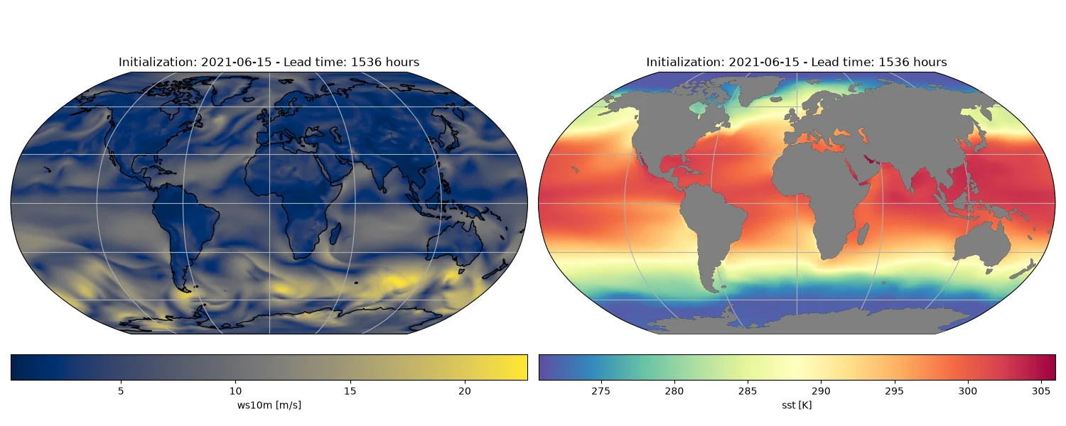
Plotting the Outputs
Let's plot some of the forecasted outputs for the atmosphere and ocean components.
import cartopy.crs as ccrs
import cartopy.feature as cfeature
import matplotlib.pyplot as plt

# lat = x_atmos_coords["lat"]
# lon = x_atmos_coords["lon"]
atmos_var, atmos_units = "ws10m", "m/s"
ocean_var, ocean_units = "sst", "K"
# atmos_var_idx = list(x_atmos_coords["variable"]).index(atmos_var)
# ocean_var_idx = list(x_ocean_coords["variable"]).index(ocean_var)
lead_time = ds.lead_time.values[-1]

plt.close("all")
# Create a Robinson projection
projection = ccrs.Robinson()

# Create a figure and axes with the specified projection
fig, axs = plt.subplots(1, 2, subplot_kw={"projection": projection}, figsize=(15, 6))

# Plot the field using pcolormesh
im = axs[0].pcolormesh(
    ds.lon.values,
    ds.lat.values,
    ds[atmos_var].sel(time=ic_date, lead_time=lead_time).values,
    transform=ccrs.PlateCarree(),
    cmap="cividis",
)

# Set title
axs[0].set_title(
    f"Initialization: {ic_date} - Lead time: {lead_time.astype('timedelta64[h]')}"
)

# Add coastlines and gridlines
axs[0].coastlines()
axs[0].gridlines()

cbar = fig.colorbar(im, ax=axs[0], orientation="horizontal", pad=0.05)
cbar.set_label(f"{atmos_var} [{atmos_units}]")

# Plot the ocean component
im = axs[1].pcolormesh(
    ds.lon.values,
    ds.lat.values,
    ds[ocean_var].sel(time=ic_date, lead_time=lead_time).values,
    transform=ccrs.PlateCarree(),
    cmap="Spectral_r",
)

axs[1].set_title(
    f"Initialization: {ic_date} - Lead time: {lead_time.astype('timedelta64[h]')}"
)

# Add coastlines and gridlines
axs[1].add_feature(cfeature.LAND, color="grey", zorder=100)
axs[1].coastlines()
axs[1].gridlines()

cbar = fig.colorbar(im, ax=axs[1], orientation="horizontal", pad=0.05)
cbar.set_label(f"{ocean_var} [{ocean_units}]")

plt.tight_layout()
plt.savefig("outputs/14_ws10m_sst_prediction.png")