IO Backend Performance

Leverage different IO backends for storing inference results.

This example explores IO backends inside Earth2Studio and how they can be used to write data to different formats / locations. The IO is a core part of any inference pipeline and depending on the desired target, can dramatically impact performance. This example will help navigate users through the use of different IO backend APIs in a simple workflow.

In this example you will learn:

• Initializing, creating arrays and writing with the Zarr IO backend
• Initializing, creating arrays and writing with the NetCDF IO backend
• Initializing and writing with the Asynchronous Non-blocking Zarr IO backend
• Discussing performance implications and strategies that can be used

Set Up

To demonstrate different IO, this example will use a simple ensemble workflow that we will manually create ourselves. One could use the built in workflow in Earth2Studio however, this will allow us to better understand the APIs.

We need the following components:

• Datasource: Pull data from the GFS data api earth2studio.data.GFS.
• Prognostic Model: Use the built in DLWP model earth2studio.models.px.DLWP.
• Perturbation Method: Use the standard Gaussian method earth2studio.perturbation.Gaussian.
• IO Backends: Use a few IO Backends including earth2studio.io.AsyncZarrBackend, earth2studio.io.NetCDF4Backend and earth2studio.io.ZarrBackend.

import os

os.makedirs("outputs", exist_ok=True)
from dotenv import load_dotenv

load_dotenv()  # TODO: make common example prep function

import torch

from earth2studio.data import GFS, DataSource, fetch_data
from earth2studio.io import AsyncZarrBackend, IOBackend, NetCDF4Backend, ZarrBackend
from earth2studio.models.px import DLWP, PrognosticModel
from earth2studio.perturbation import Gaussian, Perturbation

# Get the device
device = torch.device("cuda" if torch.cuda.is_available() else "cpu")

# Load the cBottle data source
package = DLWP.load_default_package()
model = DLWP.load_model(package)
model = model.to(device)

# Create the ERA5 data source
ds = GFS()

# Create perturbation method
pt = Gaussian()

Console output9 lines

/__w/earth2studio/earth2studio/.venv/lib/python3.13/site-packages/torch/cuda/__init__.py:64: FutureWarning: The pynvml package is deprecated. Please install nvidia-ml-py instead. If you did not install pynvml directly, please report this to the maintainers of the package that installed pynvml for you.
  import pynvml  # type: ignore[import]
WARNING[XFORMERS]: xFormers can't load C++/CUDA extensions. xFormers was built for:
    PyTorch 2.10.0+cu128 with CUDA 1208 (you have 2.13.0+cu130)
    Python  3.10.19 (you have 3.13.13)
  Please reinstall xformers (see https://github.com/facebookresearch/xformers#installing-xformers)
  Memory-efficient attention, SwiGLU, sparse and more won't be available.
  Set XFORMERS_MORE_DETAILS=1 for more details
CuPy distance computation test failed with error: cuVS >= 24.12 or pylibraft < 24.12 should be installed to use this feature

Creating a Simple Ensemble Workflow

Start with creating a simple ensemble inference workflow. This is essentially a simpler version of the built in ensemble workflow earth2studio.run.ensemble. In this case, this is for an ensemble inference workflow that will predict a 5 day forecast for Christmas 2022. Following standard Earth2Studio practices, the function accepts initialized prognostic, data source, io backend and perturbation method.

import os
import time
from datetime import datetime, timedelta

import numpy as np
from tqdm import tqdm

from earth2studio.utils.coords import map_coords, split_coords
from earth2studio.utils.time import to_time_array

times = [datetime(2024, 1, 1)]
nsteps = 20  # Assuming 6-hour time steps


def christmas_five_day_ensemble(
    times: list[datetime],
    nsteps: int,
    prognostic: PrognosticModel,
    data: DataSource,
    io: IOBackend,
    perturbation: Perturbation,
    nensemble: int = 8,
    device: str = "cuda",
) -> None:
    """Ensemble inference example"""
    # ==========================================
    # Fetch Initialization Data
    prognostic_ic = prognostic.input_coords()
    times = to_time_array(times)

    x, coords0 = fetch_data(
        source=data,
        time=times,
        variable=prognostic_ic["variable"],
        lead_time=prognostic_ic["lead_time"],
        device=device,
    )
    # ==========================================
    # ==========================================
    # Set up IO backend by pre-allocating arrays (not needed for AsyncZarrBackend)
    total_coords = prognostic.output_coords(prognostic.input_coords()).copy()
    if "batch" in total_coords:
        del total_coords["batch"]
    total_coords["time"] = times
    total_coords["lead_time"] = np.asarray(
        [
            prognostic.output_coords(prognostic.input_coords())["lead_time"] * i
            for i in range(nsteps + 1)
        ]
    ).flatten()
    total_coords.move_to_end("lead_time", last=False)
    total_coords.move_to_end("time", last=False)
    total_coords = {"ensemble": np.arange(nensemble)} | total_coords

    variables_to_save = total_coords.pop("variable")
    io.add_array(total_coords, variables_to_save)
    # ==========================================
    # ==========================================
    # Run inference
    coords = {"ensemble": np.arange(nensemble)} | coords0.copy()
    x = x.unsqueeze(0).repeat(nensemble, *([1] * x.ndim))

    # Map lat and lon if needed
    x, coords = map_coords(x, coords, prognostic_ic)

    # Perturb ensemble
    x, coords = perturbation(x, coords)

    # Create prognostic iterator
    model = prognostic.create_iterator(x, coords)

    with tqdm(
        total=nsteps + 1,
        desc="Running batch inference",
        position=1,
        leave=False,
    ) as pbar:
        for step, (x, coords) in enumerate(model):
            # Dump result to IO, split_coords separates variables to different arrays
            x, coords = map_coords(x, coords, {"variable": np.array(["t2m", "tcwv"])})
            io.write(*split_coords(x, coords))
            pbar.update(1)
            if step == nsteps:
                break
    # ==========================================


def get_folder_size(folder_path: str) -> int:
    """Get folder size in megabytes"""
    if os.path.isfile(folder_path):
        return os.path.getsize(folder_path) / (1024 * 1024)

    total_size = 0
    for dirpath, dirnames, filenames in os.walk(folder_path):
        for filename in filenames:
            file_path = os.path.join(dirpath, filename)
            total_size += os.path.getsize(file_path)
    return total_size / (1024 * 1024)

Local Storage Zarr IO

As a base line, lets run the Zarr IO backend saving it to local disk. Local IO storage is typically preferred since we can then access the data after the inference pipeline is finished using standard libraries. Chunking play an important role on performance, both with respect to compression and also when accessing data. Here we will chunk the output data based on time and lead_time

io = ZarrBackend(
    "outputs/17_io_sync.zarr",
    chunks={"time": 1, "lead_time": 1},
    backend_kwargs={"overwrite": True},
)

start_time = time.time()
christmas_five_day_ensemble(times, nsteps, model, ds, io, pt, device=device)
zarr_local_clock = time.time() - start_time

Console output52 lines

Fetching GFS data:   0%|          | 0/7 [00:00<?, ?it/s]
Fetching GFS data:  14%|█▍        | 1/7 [00:00<00:01,  5.65it/s]
Fetching GFS data: 100%|██████████| 7/7 [00:00<00:00, 38.56it/s]

Fetching GFS data:   0%|          | 0/7 [00:00<?, ?it/s]
Fetching GFS data:  14%|█▍        | 1/7 [00:00<00:00,  7.73it/s]
Fetching GFS data: 100%|██████████| 7/7 [00:00<00:00, 53.90it/s]


Running batch inference:   0%|          | 0/21 [00:00<?, ?it/s]

Running batch inference:   5%|▍         | 1/21 [00:00<00:19,  1.02it/s]

Running batch inference:  10%|▉         | 2/21 [00:02<00:20,  1.06s/it]

Running batch inference:  14%|█▍        | 3/21 [00:02<00:17,  1.06it/s]

Running batch inference:  19%|█▉        | 4/21 [00:03<00:15,  1.10it/s]

Running batch inference:  24%|██▍       | 5/21 [00:04<00:13,  1.15it/s]

Running batch inference:  29%|██▊       | 6/21 [00:05<00:13,  1.15it/s]

Running batch inference:  33%|███▎      | 7/21 [00:06<00:11,  1.18it/s]

Running batch inference:  38%|███▊      | 8/21 [00:07<00:11,  1.17it/s]

Running batch inference:  43%|████▎     | 9/21 [00:07<00:10,  1.19it/s]

Running batch inference:  48%|████▊     | 10/21 [00:08<00:09,  1.17it/s]

Running batch inference:  52%|█████▏    | 11/21 [00:09<00:08,  1.19it/s]

Running batch inference:  57%|█████▋    | 12/21 [00:10<00:07,  1.18it/s]

Running batch inference:  62%|██████▏   | 13/21 [00:11<00:06,  1.18it/s]

Running batch inference:  67%|██████▋   | 14/21 [00:12<00:06,  1.17it/s]

Running batch inference:  71%|███████▏  | 15/21 [00:13<00:05,  1.18it/s]

Running batch inference:  76%|███████▌  | 16/21 [00:13<00:04,  1.16it/s]

Running batch inference:  81%|████████  | 17/21 [00:14<00:03,  1.17it/s]

Running batch inference:  86%|████████▌ | 18/21 [00:15<00:02,  1.15it/s]

Running batch inference:  90%|█████████ | 19/21 [00:16<00:01,  1.16it/s]

Running batch inference:  95%|█████████▌| 20/21 [00:17<00:00,  1.16it/s]

Running batch inference: 100%|██████████| 21/21 [00:18<00:00,  1.17it/s]

print(f"\nLocal zarr store inference time: {zarr_local_clock}s")
print(
    f"Uncompressed zarr store size: {get_folder_size('outputs/17_io_sync.zarr'):.2f} MB"
)

Console output2 lines

Local zarr store inference time: 18.662800312042236s
Uncompressed zarr store size: 1330.78 MB

Compressed Local Storage Zarr IO

By default the Zarr IO backends will be uncompressed. In many instances this is fine, when data volumes are low. However, in instances that we are writing a very large amount of data or the data needs to get sent over the network to a remote store, compression is essential. With the standard Zarr backend, this will cause a very noticeable slow down, but note that the output store will be 3x smaller!

import zarr

io = ZarrBackend(
    "outputs/17_io_sync_compressed.zarr",
    chunks={"time": 1, "lead_time": 1},
    backend_kwargs={"overwrite": True},
    zarr_codecs=zarr.codecs.BloscCodec(
        cname="zstd", clevel=3, shuffle=zarr.codecs.BloscShuffle.shuffle
    ),  # Zarrs default
)

start_time = time.time()
christmas_five_day_ensemble(times, nsteps, model, ds, io, pt, device=device)
zarr_local_clock = time.time() - start_time

Console output52 lines

Fetching GFS data:   0%|          | 0/7 [00:00<?, ?it/s]
Fetching GFS data:  14%|█▍        | 1/7 [00:00<00:01,  5.85it/s]
Fetching GFS data: 100%|██████████| 7/7 [00:00<00:00, 39.73it/s]

Fetching GFS data:   0%|          | 0/7 [00:00<?, ?it/s]
Fetching GFS data:  14%|█▍        | 1/7 [00:00<00:01,  4.61it/s]
Fetching GFS data: 100%|██████████| 7/7 [00:00<00:00, 32.17it/s]


Running batch inference:   0%|          | 0/21 [00:00<?, ?it/s]

Running batch inference:   5%|▍         | 1/21 [00:00<00:19,  1.04it/s]

Running batch inference:  10%|▉         | 2/21 [00:02<00:21,  1.13s/it]

Running batch inference:  14%|█▍        | 3/21 [00:03<00:20,  1.16s/it]

Running batch inference:  19%|█▉        | 4/21 [00:04<00:20,  1.18s/it]

Running batch inference:  24%|██▍       | 5/21 [00:05<00:19,  1.19s/it]

Running batch inference:  29%|██▊       | 6/21 [00:07<00:18,  1.21s/it]

Running batch inference:  33%|███▎      | 7/21 [00:08<00:16,  1.21s/it]

Running batch inference:  38%|███▊      | 8/21 [00:09<00:16,  1.23s/it]

Running batch inference:  43%|████▎     | 9/21 [00:10<00:14,  1.23s/it]

Running batch inference:  48%|████▊     | 10/21 [00:12<00:13,  1.25s/it]

Running batch inference:  52%|█████▏    | 11/21 [00:13<00:12,  1.24s/it]

Running batch inference:  57%|█████▋    | 12/21 [00:14<00:11,  1.25s/it]

Running batch inference:  62%|██████▏   | 13/21 [00:15<00:09,  1.24s/it]

Running batch inference:  67%|██████▋   | 14/21 [00:17<00:08,  1.26s/it]

Running batch inference:  71%|███████▏  | 15/21 [00:18<00:07,  1.25s/it]

Running batch inference:  76%|███████▌  | 16/21 [00:19<00:06,  1.27s/it]

Running batch inference:  81%|████████  | 17/21 [00:20<00:05,  1.26s/it]

Running batch inference:  86%|████████▌ | 18/21 [00:22<00:03,  1.26s/it]

Running batch inference:  90%|█████████ | 19/21 [00:23<00:02,  1.24s/it]

Running batch inference:  95%|█████████▌| 20/21 [00:24<00:01,  1.23s/it]

Running batch inference: 100%|██████████| 21/21 [00:25<00:00,  1.22s/it]

print(f"\nLocal compressed zarr store inference time: {zarr_local_clock}s")
print(
    f"Compressed zarr store size: {get_folder_size('outputs/17_io_sync_compressed.zarr'):.2f} MB"
)

Console output2 lines

Local compressed zarr store inference time: 26.312042951583862s
Compressed zarr store size: 394.26 MB

Local Storage NetCDF IO

NetCDF offers a similar user experience but saves the output into a single netCDF file. For local storage, NetCDF it typically preferred since it keeps all outputs into a single file.

io = NetCDF4Backend("outputs/17_io_sync.nc", backend_kwargs={"mode": "w"})
start_time = time.time()
christmas_five_day_ensemble(times, nsteps, model, ds, io, pt, device=device)
nc_local_clock = time.time() - start_time

Console output24 lines

Fetching GFS data:   0%|          | 0/7 [00:00<?, ?it/s]
Fetching GFS data:  29%|██▊       | 2/7 [00:00<00:00, 16.30it/s]
Fetching GFS data: 100%|██████████| 7/7 [00:00<00:00, 54.17it/s]

Fetching GFS data:   0%|          | 0/7 [00:00<?, ?it/s]
Fetching GFS data:  43%|████▎     | 3/7 [00:00<00:00, 26.81it/s]
Fetching GFS data: 100%|██████████| 7/7 [00:00<00:00, 62.33it/s]


Running batch inference:   0%|          | 0/21 [00:00<?, ?it/s]

Running batch inference:   5%|▍         | 1/21 [00:00<00:19,  1.01it/s]

Running batch inference:  19%|█▉        | 4/21 [00:01<00:03,  4.48it/s]

Running batch inference:  33%|███▎      | 7/21 [00:01<00:01,  8.22it/s]

Running batch inference:  48%|████▊     | 10/21 [00:01<00:00, 11.36it/s]

Running batch inference:  62%|██████▏   | 13/21 [00:01<00:00, 14.77it/s]

Running batch inference:  76%|███████▌  | 16/21 [00:01<00:00, 16.76it/s]

Running batch inference:  90%|█████████ | 19/21 [00:01<00:00, 19.40it/s]

print(f"\nLocal netcdf store inference time: {nc_local_clock}s")
print(
    f"Uncompressed zarr store size: {get_folder_size('outputs/17_io_sync.nc'):.2f} MB"
)

Console output2 lines

Local netcdf store inference time: 2.0828278064727783s
Uncompressed zarr store size: 1330.79 MB

In Memory Zarr IO

One way we can speed up IO is to save outputs to in-memory stores. In-memory stores more limited in size depending on the hardware being used. Also one needs to be careful with in memory stores, once the Python object is deleted the data is gone.

io = ZarrBackend(
    chunks={"time": 1, "lead_time": 1}, backend_kwargs={"overwrite": True}
)  # Not path = in memory for Zarr
start_time = time.time()
christmas_five_day_ensemble(times, nsteps, model, ds, io, pt, device=device)
zarr_memory_clock = time.time() - start_time

Console output52 lines

Fetching GFS data:   0%|          | 0/7 [00:00<?, ?it/s]
Fetching GFS data:  43%|████▎     | 3/7 [00:00<00:00, 29.28it/s]
Fetching GFS data: 100%|██████████| 7/7 [00:00<00:00, 68.15it/s]

Fetching GFS data:   0%|          | 0/7 [00:00<?, ?it/s]
Fetching GFS data:  14%|█▍        | 1/7 [00:00<00:00,  6.88it/s]
Fetching GFS data: 100%|██████████| 7/7 [00:00<00:00, 47.28it/s]


Running batch inference:   0%|          | 0/21 [00:00<?, ?it/s]

Running batch inference:   5%|▍         | 1/21 [00:00<00:13,  1.45it/s]

Running batch inference:  10%|▉         | 2/21 [00:01<00:13,  1.42it/s]

Running batch inference:  14%|█▍        | 3/21 [00:02<00:12,  1.42it/s]

Running batch inference:  19%|█▉        | 4/21 [00:02<00:12,  1.40it/s]

Running batch inference:  24%|██▍       | 5/21 [00:03<00:11,  1.41it/s]

Running batch inference:  29%|██▊       | 6/21 [00:04<00:10,  1.40it/s]

Running batch inference:  33%|███▎      | 7/21 [00:04<00:09,  1.41it/s]

Running batch inference:  38%|███▊      | 8/21 [00:05<00:09,  1.37it/s]

Running batch inference:  43%|████▎     | 9/21 [00:06<00:08,  1.39it/s]

Running batch inference:  48%|████▊     | 10/21 [00:07<00:07,  1.39it/s]

Running batch inference:  52%|█████▏    | 11/21 [00:07<00:07,  1.41it/s]

Running batch inference:  57%|█████▋    | 12/21 [00:08<00:06,  1.40it/s]

Running batch inference:  62%|██████▏   | 13/21 [00:09<00:05,  1.39it/s]

Running batch inference:  67%|██████▋   | 14/21 [00:10<00:05,  1.37it/s]

Running batch inference:  71%|███████▏  | 15/21 [00:10<00:04,  1.38it/s]

Running batch inference:  76%|███████▌  | 16/21 [00:11<00:03,  1.38it/s]

Running batch inference:  81%|████████  | 17/21 [00:12<00:02,  1.39it/s]

Running batch inference:  86%|████████▌ | 18/21 [00:12<00:02,  1.38it/s]

Running batch inference:  90%|█████████ | 19/21 [00:13<00:01,  1.40it/s]

Running batch inference:  95%|█████████▌| 20/21 [00:14<00:00,  1.38it/s]

Running batch inference: 100%|██████████| 21/21 [00:15<00:00,  1.40it/s]

print(f"\nIn memory zarr store inference time: {zarr_memory_clock}s")

Console output1 line

In memory zarr store inference time: 15.410285949707031s

Compressed Local Async Zarr IO

The async Zarr IO backend is an advanced IO backend designed to offer async Zarr 3.0 writes to in-memory, local and remote data stores. This data source is ideal when large volumes of data are needed to be written and the users want to mask the IO with the forward execution of the model.

Because this IO backend relies on both async and multi-threading, it has a different initialization pattern than others. The main difference being that this backend does not use the add_array API, rather users specify parallel_coords in the constructor that denote coords that slices will be written to during inference. Typically this might be time, lead_time and ensemble.

parallel_coords = {
    "time": np.array(times, dtype=np.datetime64),
    "lead_time": np.array(
        [timedelta(hours=6 * i) for i in range(nsteps + 1)], dtype=np.timedelta64
    ),
}
io = AsyncZarrBackend(
    "outputs/17_io_async.zarr",
    parallel_coords=parallel_coords,
    zarr_codecs=zarr.codecs.BloscCodec(
        cname="zstd", clevel=3, shuffle=zarr.codecs.BloscShuffle.shuffle
    ),
)
start_time = time.time()
christmas_five_day_ensemble(times, nsteps, model, ds, io, pt, device=device)
zarr_async_clock = time.time() - start_time

Console output52 lines

Fetching GFS data:   0%|          | 0/7 [00:00<?, ?it/s]
Fetching GFS data:  14%|█▍        | 1/7 [00:00<00:00,  7.97it/s]
Fetching GFS data: 100%|██████████| 7/7 [00:00<00:00, 55.34it/s]

Fetching GFS data:   0%|          | 0/7 [00:00<?, ?it/s]
Fetching GFS data:  14%|█▍        | 1/7 [00:00<00:00,  7.20it/s]
Fetching GFS data: 100%|██████████| 7/7 [00:00<00:00, 46.93it/s]


Running batch inference:   0%|          | 0/21 [00:00<?, ?it/s]

Running batch inference:   5%|▍         | 1/21 [00:00<00:04,  4.90it/s]

Running batch inference:  10%|▉         | 2/21 [00:00<00:05,  3.39it/s]

Running batch inference:  14%|█▍        | 3/21 [00:00<00:05,  3.15it/s]

Running batch inference:  19%|█▉        | 4/21 [00:01<00:05,  2.87it/s]

Running batch inference:  24%|██▍       | 5/21 [00:01<00:05,  2.88it/s]

Running batch inference:  29%|██▊       | 6/21 [00:02<00:05,  2.83it/s]

Running batch inference:  33%|███▎      | 7/21 [00:02<00:04,  2.94it/s]

Running batch inference:  38%|███▊      | 8/21 [00:02<00:04,  2.88it/s]

Running batch inference:  43%|████▎     | 9/21 [00:03<00:04,  2.96it/s]

Running batch inference:  48%|████▊     | 10/21 [00:03<00:03,  2.94it/s]

Running batch inference:  52%|█████▏    | 11/21 [00:03<00:03,  2.96it/s]

Running batch inference:  57%|█████▋    | 12/21 [00:04<00:03,  2.92it/s]

Running batch inference:  62%|██████▏   | 13/21 [00:04<00:02,  2.96it/s]

Running batch inference:  67%|██████▋   | 14/21 [00:04<00:02,  2.94it/s]

Running batch inference:  71%|███████▏  | 15/21 [00:05<00:02,  2.94it/s]

Running batch inference:  76%|███████▌  | 16/21 [00:05<00:01,  2.93it/s]

Running batch inference:  81%|████████  | 17/21 [00:05<00:01,  2.98it/s]

Running batch inference:  86%|████████▌ | 18/21 [00:06<00:01,  2.96it/s]

Running batch inference:  90%|█████████ | 19/21 [00:06<00:00,  2.94it/s]

Running batch inference:  95%|█████████▌| 20/21 [00:06<00:00,  2.90it/s]

Running batch inference: 100%|██████████| 21/21 [00:07<00:00,  2.92it/s]

print(f"\nAsync zarr store inference time: {zarr_async_clock}s")
print(
    f"Compressed async zarr store size: {get_folder_size('outputs/17_io_async.zarr'):.2f} MB"
)

Console output2 lines

Async zarr store inference time: 7.504284858703613s
Compressed async zarr store size: 394.26 MB

Compressed Local Non-Blocking Async Zarr IO

That was faster than the normal Zarr method, even the uncompressed version making it comparable to NetCDF, but we can still improve with this IO backend. A unique feature of this particular backend is running in non-blocking mode, namely IO writes will be placed onto other threads. Users do need to be careful with this to both ensure data is not mutated while the IO backend is working to move the data off the GPU, but also to make sure to wait for write threads to finish before the object is deleted.

Note that this backend allows Zarr to be comparable to uncompressed NetCDF even 3x compression!

io = AsyncZarrBackend(
    "outputs/17_io_nonblocking_async.zarr",
    parallel_coords=parallel_coords,
    blocking=False,
    zarr_codecs=zarr.codecs.BloscCodec(
        cname="zstd", clevel=3, shuffle=zarr.codecs.BloscShuffle.shuffle
    ),
)
start_time = time.time()
christmas_five_day_ensemble(times, nsteps, model, ds, io, pt, device=device)
# IMPORTANT: Make sure to call close to ensure IO backend threads have finished!
io.close()
zarr_nonblocking_async_clock = time.time() - start_time

Console output30 lines

Fetching GFS data:   0%|          | 0/7 [00:00<?, ?it/s]
Fetching GFS data:  29%|██▊       | 2/7 [00:00<00:00, 13.60it/s]
Fetching GFS data: 100%|██████████| 7/7 [00:00<00:00, 46.18it/s]

Fetching GFS data:   0%|          | 0/7 [00:00<?, ?it/s]
Fetching GFS data:  14%|█▍        | 1/7 [00:00<00:00,  7.60it/s]
Fetching GFS data: 100%|██████████| 7/7 [00:00<00:00, 50.54it/s]


Running batch inference:   0%|          | 0/21 [00:00<?, ?it/s]

Running batch inference:  10%|▉         | 2/21 [00:00<00:01, 12.95it/s]

Running batch inference:  19%|█▉        | 4/21 [00:00<00:02,  6.60it/s]

Running batch inference:  29%|██▊       | 6/21 [00:00<00:02,  5.73it/s]

Running batch inference:  38%|███▊      | 8/21 [00:01<00:02,  5.51it/s]

Running batch inference:  48%|████▊     | 10/21 [00:01<00:02,  5.46it/s]

Running batch inference:  57%|█████▋    | 12/21 [00:02<00:01,  5.49it/s]

Running batch inference:  67%|██████▋   | 14/21 [00:02<00:01,  5.51it/s]

Running batch inference:  76%|███████▌  | 16/21 [00:02<00:00,  5.35it/s]

Running batch inference:  86%|████████▌ | 18/21 [00:03<00:00,  5.02it/s]

Running batch inference:  95%|█████████▌| 20/21 [00:03<00:00,  4.96it/s]

print(
    f"\nNon-blocking async zarr store inference time: {zarr_nonblocking_async_clock}s"
)
print(
    f"Compressed non-blocking async zarr store size: {get_folder_size('outputs/17_io_nonblocking_async.zarr'):.2f} MB"
)

Console output2 lines

Non-blocking async zarr store inference time: 4.472781658172607s
Compressed non-blocking async zarr store size: 394.25 MB

Remote Non-Blocking Async Zarr IO

This IO backend can be further customized by changing the Fsspec Filesystem used by the Zarr store which can be controlled via the fs_factory parameter. Note that this is a factory method, the IO backend will need to create multiple instances of the file system. Some examples that may be of interest are:

• from fsspec.implementations.local import LocalFileSystem (Default, local store)
• from fsspec.implementations.memory import MemoryFileSystem (in-memory store)
• from s3fs import S3FileSystem (Remote S3 store)

For sake of example, lets have a look at writing to a remote store would require. Compression is a must in this instances, since we need to minimize the data transfer over the network. The file system factory is set to S3 with the appropiate credentials in a partial callable object. Lastly we can increase the max number of thread workers with the pool_size parameter to further boost performance.

import functools

import s3fs

if "S3FS_KEY" in os.environ and "S3FS_SECRET" in os.environ:
    # Remember, needs to be a callable
    fs_factory = functools.partial(
        s3fs.S3FileSystem,
        key=os.environ["S3FS_KEY"],
        secret=os.environ["S3FS_SECRET"],
        client_kwargs={"endpoint_url": os.environ.get("S3FS_ENDPOINT", None)},
        asynchronous=True,
    )
    io = AsyncZarrBackend(
        "earth2studio/ci/example/17_io_async.zarr",
        parallel_coords=parallel_coords,
        fs_factory=fs_factory,
        blocking=False,
        pool_size=16,
        zarr_codecs=zarr.codecs.BloscCodec(
            cname="zstd", clevel=3, shuffle=zarr.codecs.BloscShuffle.shuffle
        ),
    )
    christmas_five_day_ensemble(times, 4, model, ds, io, pt, device=device)
    # IMPORTANT: Make sure to call close to ensure IO backend threads have finished!
    io.close()

    # To clean up the zarr store you can use
    # fs = s3fs.S3FileSystem(
    #     key=os.environ["S3FS_KEY"],
    #     secret=os.environ["S3FS_SECRET"],
    #     client_kwargs={"endpoint_url": os.environ.get("S3FS_ENDPOINT", None)},
    # )
    # fs.rm("earth2studio/ci/example/17_io_async.zarr", recursive=True)

Post-Processing

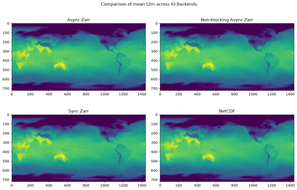
Lastly, we can plot the each of the local Zarr stores to verify that indeed they are the same.

import matplotlib.pyplot as plt
import xarray as xr

# Load the datasets
ds_async = xr.open_zarr("outputs/17_io_async.zarr", consolidated=False)
ds_nonblocking = xr.open_zarr(
    "outputs/17_io_nonblocking_async.zarr", consolidated=False
)
ds_sync = xr.open_zarr("outputs/17_io_sync.zarr")
ds_nc = xr.open_dataset("outputs/17_io_sync.nc")

# Create a 2x2 subplot grid
fig, axes = plt.subplots(2, 2, figsize=(12, 8))
fig.suptitle("Comparison of mean t2m across IO Backends")

# Plot t2m from each dataset
axes[0, 0].imshow(
    ds_async.t2m.isel(time=0, lead_time=8).mean(dim="ensemble"), vmin=250, vmax=320
)
axes[0, 0].set_title("Async Zarr")

axes[0, 1].imshow(
    ds_nonblocking.t2m.isel(time=0, lead_time=8).mean(dim="ensemble"),
    vmin=250,
    vmax=320,
)
axes[0, 1].set_title("Non-blocking Async Zarr")

axes[1, 0].imshow(
    ds_sync.t2m.isel(time=0, lead_time=8).mean(dim="ensemble"), vmin=250, vmax=320
)
axes[1, 0].set_title("Sync Zarr")

axes[1, 1].imshow(
    ds_nc.t2m.isel(time=0, lead_time=8).mean(dim="ensemble"), vmin=250, vmax=320
)
axes[1, 1].set_title("NetCDF")

plt.tight_layout()
plt.savefig("outputs/17_io_performance.jpg", bbox_inches="tight")

---

Download Python sourceDownload Jupyter notebookexecuted in 109.3s

Execution profile

Runtime telemetry

Total runtime1m 49s

Execution environment

CPUAMD EPYC 7313P 16-Core Processor

GPUNVIDIA H100 PCIe · 79.6 GiB

System RAM58.5 GiB

PlatformLinux 6.8.0-136-generic

Python3.13.13

GPU driver / CUDADriver 595.84 · CUDA support 13.2