Composable Model Composition (LJ + Ewald)

Real force fields for ionic systems combine multiple physical contributions:

• Short-range repulsion / dispersion — described by Lennard-Jones (or Born–Mayer) pair potentials that capture electron-cloud overlap and van der Waals attraction.

• Long-range Coulomb interactions — must be treated with Ewald summation or PME to avoid artifacts from naive truncation.

nvalchemi lets you combine any two BaseModelMixin-compatible models with the + operator:

combined = lj_model + ewald_model

The result is an ComposableModelWrapper that calls each sub-model in sequence and sums their energies, forces, and stresses element-wise. A single shared ModelConfig instance propagates flags like compute_stresses to every sub-model automatically.

This example:

• Builds a simple charge-neutral ionic fluid (alternating +1/−1 particles on a cubic lattice, inspired by a primitive model electrolyte).

• Combines a Lennard-Jones short-range model with an Ewald long-range model.

• Shows that setting combined.model_config.compute_stresses = True automatically activates stress computation in both sub-models.

• Demonstrates make_neighbor_hooks() which returns the single hook needed for the composite model (using the maximum cutoff across all sub-models).

• Runs 200 NVT steps and logs the combined (LJ + Coulomb) energy.

Key concepts demonstrated

• model_a + model_b syntax — creates a flat ComposableModelWrapper.

• Shared ModelConfig — mutating combined.model_config.compute_forces = False disables forces in every sub-model with a single assignment.

• make_neighbor_hooks() — returns a list with one correctly-configured NeighborListHook.

• Chaining three or more models — a + b + c flattens into one wrapper.

from __future__ import annotations

import logging
import os

import torch

from nvalchemi.data import AtomicData, Batch
from nvalchemi.dynamics import NVTLangevin
from nvalchemi.dynamics.hooks import LoggingHook, WrapPeriodicHook
from nvalchemi.models.ewald import EwaldModelWrapper
from nvalchemi.models.lj import LennardJonesModelWrapper

logging.basicConfig(level=logging.INFO)

Building the composite model

We model a primitive-electrolyte ionic fluid: equal numbers of cations (+1 e) and anions (−1 e) interacting via LJ + Coulomb. This is the simplest model for a molten salt or ionic solution.

LJ parameters — both species use the same σ and ε (symmetric primitive model), representing hard-core repulsion at short range.

Ewald model — handles the long-range 1/r Coulomb tail. The real-space cutoff must be the same for both models (or the Ewald cutoff may be larger); the additive wrapper automatically takes the maximum.

LJ_EPSILON = 0.05  # eV   — moderate well depth for a "soft" ion
LJ_SIGMA = 2.50  # Å    — ionic diameter
LJ_CUTOFF = 8.0  # Å    — short-range cutoff
EWALD_CUTOFF = 8.0  # Å    — Ewald real-space cutoff (same here)
MAX_NEIGHBORS = 128

lj_model = LennardJonesModelWrapper(
    epsilon=LJ_EPSILON,
    sigma=LJ_SIGMA,
    cutoff=LJ_CUTOFF,
    max_neighbors=MAX_NEIGHBORS,
)

ewald_model = EwaldModelWrapper(
    cutoff=EWALD_CUTOFF,
    accuracy=1e-6,
    max_neighbors=MAX_NEIGHBORS,
)

# Combine with the + operator.  The result is an ComposableModelWrapper that
# runs both sub-models and sums their energies/forces/stresses.
combined = lj_model + ewald_model

print(f"Combined model type: {type(combined).__name__}")
print(f"Sub-models: {[type(m).__name__ for m in combined.models]}")

Combined model type: ComposableModelWrapper
Sub-models: ['LennardJonesModelWrapper', 'EwaldModelWrapper']

Shared ModelConfig propagation

Setting any flag on combined.model_config propagates to both sub-models through a shared reference — no need to set it on each one separately.

For example, to disable force computation (e.g. for energy-only evaluation):

combined.model_config.compute_forces = False

Or to enable stress computation for NPT (requires the batch to have stress storage pre-allocated — standard NPT dynamics handles this automatically):

combined.model_config.compute_stresses = True assert lj_model.model_config.compute_stresses is True # propagated assert ewald_model.model_config.compute_stresses is True

# Demonstrate propagation using compute_forces (safe to toggle without a
# pre-allocated stress buffer).
combined.model_config.compute_forces = True
assert lj_model.model_config.compute_forces is True
assert ewald_model.model_config.compute_forces is True
print("model_config propagated to both sub-models ✓")

# The synthesised ModelCard reflects the union of sub-model capabilities.
card = combined.model_card
print(
    f"Combined neighbor config: cutoff={card.neighbor_config.cutoff} Å, "
    f"format={card.neighbor_config.format.name}"
)

model_config propagated to both sub-models ✓
Combined neighbor config: cutoff=8.0 Å, format=MATRIX

System: primitive electrolyte on a cubic lattice

Place N_SIDE³ ions on a simple-cubic lattice, alternating +1 / −1 charges (like NaCl but with identical mass and LJ parameters for both species). The system is charge-neutral by construction (equal number of each sign).

N_SIDE = 4  # 4³ = 64 ions
T_INIT = 300.0  # K  (room temperature — keeps ions near the LJ+Coulomb minimum)
M_ION = 23.0  # amu (sodium-like mass for both species)
KB_EV = 8.617333262e-5  # eV/K

# Lattice spacing = LJ equilibrium distance r_min = 2^(1/6) σ.
# At this spacing the LJ force is zero; the net Coulomb force is also zero
# by Madelung symmetry.  Both sub-models combined therefore produce near-zero
# forces at the initial lattice sites, giving a well-defined starting point.
r_min = 2 ** (1 / 6) * LJ_SIGMA  # ≈ 2.806 Å
box_size = N_SIDE * r_min

coords = torch.arange(N_SIDE, dtype=torch.float32) * r_min
gx, gy, gz = torch.meshgrid(coords, coords, coords, indexing="ij")
positions = torch.stack([gx.flatten(), gy.flatten(), gz.flatten()], dim=-1)
n_atoms = positions.shape[0]  # 64

# Checkerboard charge pattern: +1 if (ix+iy+iz) is even, −1 otherwise.
ix = torch.arange(N_SIDE).repeat_interleave(N_SIDE * N_SIDE)
iy = torch.arange(N_SIDE).repeat(N_SIDE).repeat_interleave(N_SIDE)
iz = torch.arange(N_SIDE).repeat(N_SIDE * N_SIDE)
parity = (ix + iy + iz) % 2  # 0 or 1
charges_1d = torch.where(parity == 0, torch.tensor(1.0), torch.tensor(-1.0))
charges = charges_1d.unsqueeze(-1)  # (N, 1) — required shape for AtomicData

atomic_numbers = torch.full((n_atoms,), 11, dtype=torch.long)  # all "Na"

kT = KB_EV * T_INIT
torch.manual_seed(1)
v_scale = (kT / M_ION) ** 0.5
velocities = torch.randn(n_atoms, 3) * v_scale
velocities -= velocities.mean(dim=0, keepdim=True)

cell = torch.eye(3).unsqueeze(0) * box_size

data = AtomicData(
    positions=positions,
    atomic_numbers=atomic_numbers,
    node_charges=charges,  # (N, 1)
    forces=torch.zeros(n_atoms, 3),
    energies=torch.zeros(1, 1),
    cell=cell,
    pbc=torch.tensor([[True, True, True]]),
)
data.add_node_property("velocities", velocities)

batch = Batch.from_data_list([data])
print(
    f"\nSystem: {n_atoms} ions, box={box_size:.2f} Å, "
    f"net charge={charges_1d.sum().item():.0f} e, T_init={T_INIT} K"
)

System: 64 ions, box=11.22 Å, net charge=0 e, T_init=300.0 K

NVT simulation with the composite model

make_neighbor_hooks() returns a list containing exactly one NeighborListHook configured for the combined model’s effective cutoff (max of all sub-model cutoffs). Registering this single hook is all that is needed — the neighbor data is shared between both sub-models via prepare_neighbors_for_model().

nvt = NVTLangevin(
    model=combined,
    dt=0.5,  # fs — conservative timestep for stiff Coulomb forces
    temperature=T_INIT,
    friction=0.5,  # ps⁻¹ — moderate coupling keeps ions near equilibrium
    n_steps=200,
    random_seed=99,
)

for hook in combined.make_neighbor_hooks():
    nvt.register_hook(hook)
nvt.register_hook(WrapPeriodicHook())

Running and logging

COMBINED_LOG = "lj_ewald_combined.csv"

with LoggingHook(backend="csv", log_path=COMBINED_LOG, frequency=20) as log_hook:
    nvt.register_hook(log_hook)
    batch = nvt.run(batch)

print(f"\nNVT (LJ + Ewald) completed {nvt.step_count} steps. Log → {COMBINED_LOG}")

NVT (LJ + Ewald) completed 200 steps. Log → lj_ewald_combined.csv

Results — combined energy and temperature

import csv  # noqa: E402

rows = []
try:
    with open(COMBINED_LOG) as f:
        rows = list(csv.DictReader(f))
except FileNotFoundError:
    print(f"Log file {COMBINED_LOG} not found — skipping summary.")

if rows:
    print(f"\n{'step':>6}  {'energy (eV)':>14}  {'temperature (K)':>16}")
    print("-" * 42)
    for row in rows:
        print(
            f"{int(float(row['step'])):6d}  "
            f"{float(row['energy']):14.4f}  "
            f"{float(row['temperature']):16.2f}"
        )

  step     energy (eV)   temperature (K)
------------------------------------------
     0       -303.0969            330.25
    20       -303.1187            235.23
    40       -303.7548            298.41
    60       -304.5198            336.35
    80       -305.8333            304.69
   100       -306.2866            311.78
   120       -306.9965            368.30
   140       -307.5663            271.23
   160       -308.4895            249.19
   180       -308.7933            295.91

Extending the composition

The + operator is associative and chains are automatically flattened. For example, to add a D3 dispersion correction on top:

from nvalchemi.models.dftd3 import DFTD3ModelWrapper

dftd3 = DFTD3ModelWrapper(cutoff=10.0, functional="pbe", ...)
full_model = lj_model + ewald_model + dftd3
# full_model.models has three entries (not nested wrappers)

Or to attach an MLIP and a long-range correction:

mlip_model = MACEModelWrapper.from_file("model.pt", ...)
full_model = mlip_model + dftd3 + ewald_model

A single call to full_model.make_neighbor_hooks() returns the one hook needed for the combined system, automatically choosing the maximum cutoff and the most general neighbor format (MATRIX if any sub-model requires it).

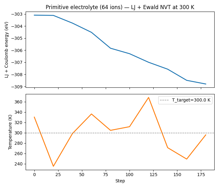
Optional plot — energy vs step

if os.getenv("NVALCHEMI_PLOT", "0") == "1" and rows:
    try:
        import matplotlib.pyplot as plt

        steps = [int(float(r["step"])) for r in rows]
        energies = [float(r["energy"]) for r in rows]
        temps = [float(r["temperature"]) for r in rows]

        fig, (ax1, ax2) = plt.subplots(2, 1, figsize=(7, 6), sharex=True)
        ax1.plot(steps, energies, lw=2)
        ax1.set_ylabel("LJ + Coulomb energy (eV)")
        ax1.set_title(
            f"Primitive electrolyte ({n_atoms} ions) — LJ + Ewald NVT at {T_INIT:.0f} K"
        )

        ax2.plot(steps, temps, lw=2, color="tab:orange")
        ax2.axhline(T_INIT, color="gray", ls="--", lw=1, label=f"T_target={T_INIT} K")
        ax2.set_xlabel("Step")
        ax2.set_ylabel("Temperature (K)")
        ax2.legend()

        fig.tight_layout()
        plt.savefig("lj_ewald_combined.png", dpi=150)
        print("Saved lj_ewald_combined.png")
        plt.show()
    except ImportError:
        print("matplotlib not available — skipping plot.")

Saved lj_ewald_combined.png