Microcanonical (NVE) Molecular Dynamics#

The NVE ensemble (constant Number of atoms, Volume, and Energy) is the most fundamental MD ensemble. The total energy E = KE + PE is conserved by the equations of motion, so any drift in E is a measure of integration error.

This example:

Builds a periodic simple-cubic argon crystal in a cubic box.
Initialises velocities from a Maxwell-Boltzmann distribution at T = 50 K.
Runs 200 steps of NVE MD with the Lennard-Jones potential.
Tracks potential energy, kinetic energy, and total energy at regular intervals to demonstrate energy conservation.
Optionally plots E(t) vs step (set NVALCHEMI_PLOT=1 to enable).

A WrapPeriodicHook folds atom positions back into the unit cell at every step, preventing coordinates from drifting far from the origin. An EnergyDriftMonitorHook warns if the per-atom-per-step energy drift exceeds a threshold.

from __future__ import annotations

import csv
import logging
import os

import torch

from nvalchemi.data import AtomicData, Batch
from nvalchemi.dynamics import NVE
from nvalchemi.dynamics.hooks import (
    EnergyDriftMonitorHook,
    LoggingHook,
    NeighborListHook,
    WrapPeriodicHook,
)
from nvalchemi.models.lj import LennardJonesModelWrapper

logging.basicConfig(level=logging.INFO)

LJ model and argon parameters#

Same Lennard-Jones parameters as the geometry-optimization example. Argon is well-described by LJ: it is a noble gas with purely dispersion interactions, no covalent bonding, and well-characterised ε and σ values from scattering experiments.

epsilon = 0.0104 eV — potential well depth
sigma = 3.40 Å — zero-crossing distance
r_min = 2^(1/6) σ ≈ 3.82 Å — equilibrium pair distance

LJ_EPSILON = 0.0104  # eV
LJ_SIGMA = 3.40  # Å
LJ_CUTOFF = 8.5  # Å
MAX_NEIGHBORS = 64  # periodic system can have more neighbours than a cluster

model = LennardJonesModelWrapper(
    epsilon=LJ_EPSILON,
    sigma=LJ_SIGMA,
    cutoff=LJ_CUTOFF,
    max_neighbors=MAX_NEIGHBORS,
)

Building a periodic argon crystal#

Place N_SIDE³ argon atoms on a simple-cubic lattice inside a cubic simulation box with periodic boundary conditions. The box side length is chosen so the lattice constant equals r_min (the LJ equilibrium distance), giving a near-equilibrium starting configuration.

Velocities are sampled from a Maxwell-Boltzmann distribution at T = 50 K. nvalchemi stores velocities in units of sqrt(eV/amu). The thermal speed scale is simply:

v_scale = sqrt(kT / m) [sqrt(eV/amu)]

where kT is in eV and m is in amu. No additional conversion factor is needed because the unit is defined so that KE = 0.5 * m * v² is directly in eV. The centre-of-mass velocity is zeroed to remove any net drift.

N_SIDE = 3  # atoms per side → N_SIDE³ = 27 atoms total
T_INIT = 50.0  # K
KB_EV = 8.617333262e-5  # eV/K
M_AR = 39.948  # amu (argon atomic mass)

kT = KB_EV * T_INIT  # eV

_R_MIN = 2 ** (1 / 6) * LJ_SIGMA  # ≈ 3.82 Å
spacing = _R_MIN
box_size = N_SIDE * spacing  # Å

# Build simple-cubic lattice positions
coords = torch.arange(N_SIDE, dtype=torch.float32) * spacing
gx, gy, gz = torch.meshgrid(coords, coords, coords, indexing="ij")
positions = torch.stack([gx.flatten(), gy.flatten(), gz.flatten()], dim=-1)
n_atoms = positions.shape[0]

# Sample Maxwell-Boltzmann velocities
torch.manual_seed(42)
v_scale = (kT / M_AR) ** 0.5  # sqrt(eV/amu)
velocities = torch.randn(n_atoms, 3) * v_scale

# Zero the centre-of-mass velocity to remove net translation
velocities -= velocities.mean(dim=0, keepdim=True)

data = AtomicData(
    positions=positions,
    atomic_numbers=torch.full((n_atoms,), 18, dtype=torch.long),  # Argon Z=18
    forces=torch.zeros(n_atoms, 3),
    energies=torch.zeros(1, 1),
    cell=torch.eye(3).unsqueeze(0) * box_size,
    pbc=torch.tensor([[True, True, True]]),
)
data.add_node_property("velocities", velocities)

batch = Batch.from_data_list([data])
print(
    f"System: {n_atoms} Ar atoms, box={box_size:.2f} Å, "
    f"T_init≈{T_INIT} K, v_scale={v_scale:.6f} sqrt(eV/amu)"
)

System: 27 Ar atoms, box=11.45 Å, T_init≈50.0 K, v_scale=0.010385 sqrt(eV/amu)

NVE integrator setup#

NVE integrates Newton’s equations with the velocity-Verlet algorithm. dt=1.0 fs is a safe timestep for argon near room temperature with LJ forces.

Three hooks are registered:

NeighborListHook — rebuilds the dense neighbor matrix when any atom has moved more than skin/2 since the last build (Verlet skin = 0.5 Å by default, so rebuild triggers at >0.25 Å displacement). A larger skin reduces rebuild frequency (faster) at the cost of a larger memory footprint; smaller skin is more memory-efficient but rebuilds more often.
WrapPeriodicHook — folds positions back into the simulation cell after each position update.
EnergyDriftMonitorHook — checks per-atom-per-step drift every step and emits a warning if it exceeds 1e-4 eV.

nve = NVE(model=model, dt=1.0, n_steps=200)

nve.register_hook(NeighborListHook(model.model_card.neighbor_config))
nve.register_hook(WrapPeriodicHook())
nve.register_hook(
    EnergyDriftMonitorHook(
        threshold=1e-4,
        metric="per_atom_per_step",
        action="warn",
        frequency=10,
    )
)

Running NVE and tracking energy conservation#

LoggingHook records energy (PE) and temperature per graph to a CSV file every 10 steps. KE is not logged directly, but can be recovered from temperature post-run:

KE = (3/2) · N · k_B · T

using the equipartition theorem (3 translational DOF per atom). All computation and I/O run asynchronously on a background thread.

NVE_LOG = "nve_energy.csv"

with LoggingHook(backend="csv", log_path=NVE_LOG, frequency=10) as log_hook:
    nve.register_hook(log_hook)
    batch = nve.run(batch)

print(f"NVE completed {nve.step_count} steps. Log: {NVE_LOG}")

NVE completed 200 steps. Log: nve_energy.csv

Results — energy conservation#

Read the CSV written by LoggingHook and reconstruct (step, KE, PE, E_total). LoggingHook logs energy (PE) and temperature per graph; KE follows from the equipartition theorem. For LJ argon at 50 K with dt=1 fs, total energy drift is typically in the sub-meV range over a few hundred steps.

energy_log = []  # (step, KE, PE, E_total)
try:
    with open(NVE_LOG) as f:
        for row in csv.DictReader(f):
            step = int(float(row["step"]))
            pe = float(row["energy"])
            T = float(row["temperature"])
            ke = 1.5 * n_atoms * KB_EV * T
            energy_log.append((step, ke, pe, ke + pe))
except FileNotFoundError:
    print(f"Log file {NVE_LOG} not found — skipping energy analysis.")

if energy_log:
    etot_vals = [r[3] for r in energy_log]
    n_log = len(energy_log)
    indices = [0, n_log // 2, n_log - 1]

    print(f"\n{'step':>6}  {'KE (eV)':>12}  {'PE (eV)':>12}  {'E_total (eV)':>14}")
    print("-" * 50)
    for idx in indices:
        s, ke, pe, et = energy_log[idx]
        print(f"{s:6d}  {ke:12.6f}  {pe:12.6f}  {et:14.6f}")

    e0 = etot_vals[0]
    drift = max(abs(e - e0) for e in etot_vals)
    drift_per_atom_per_step = drift / (n_atoms * nve.step_count)
    print(f"\nMax |ΔE_total| over trajectory: {drift:.6f} eV")
    print(
        f"Per-atom-per-step drift:         {drift_per_atom_per_step:.2e} eV/atom/step"
    )

  step       KE (eV)       PE (eV)    E_total (eV)
--------------------------------------------------
     0      0.177259     -1.345169       -1.167910
   100      0.176638     -1.376082       -1.199444
   190      0.200026     -1.400666       -1.200640

Max |ΔE_total| over trajectory: 0.034578 eV
Per-atom-per-step drift:         6.40e-06 eV/atom/step

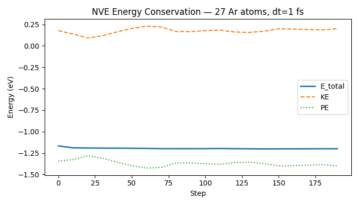
Optional plot — total energy vs step#

Set the environment variable NVALCHEMI_PLOT=1 to generate a matplotlib figure of E_total, KE, and PE vs simulation step.

if os.getenv("NVALCHEMI_PLOT", "0") == "1" and energy_log:
    import matplotlib.pyplot as plt

    steps = [r[0] for r in energy_log]
    fig, ax = plt.subplots(figsize=(7, 4))
    ax.plot(steps, [r[3] for r in energy_log], label="E_total", lw=2)
    ax.plot(steps, [r[1] for r in energy_log], label="KE", lw=1.5, ls="--")
    ax.plot(steps, [r[2] for r in energy_log], label="PE", lw=1.5, ls=":")
    ax.set_xlabel("Step")
    ax.set_ylabel("Energy (eV)")
    ax.set_title(f"NVE Energy Conservation — {n_atoms} Ar atoms, dt=1 fs")
    ax.legend()
    fig.tight_layout()
    plt.savefig("nve_energy_conservation.png", dpi=150)
    print("Saved nve_energy_conservation.png")
    plt.show()

NVE Energy Conservation — 27 Ar atoms, dt=1 fs

Saved nve_energy_conservation.png

Total running time of the script: (0 minutes 0.840 seconds)

Gallery generated by Sphinx-Gallery