CBottle Super Resolution#

Climate in a Bottle (cBottle) super resolution workflows for global weather.

This example will demonstrate the cBottle diffusion model for super resolution of global weather data. The CBottleSR model takes low-resolution climate data and generates high-resolution outputs using a diffusion-based approach.

For more information on cBottle see:

https://arxiv.org/abs/2505.06474v1

In this example you will learn:

Performing super resolution on synthetic data from the cBottle data source
Performing super resolution on ERA5 data after infilling with cBottle
Post-processing and visualizing super-resolution results

Set Up#

For this example we will use the cBottle data source, infill diagnostic, and the CBottleSR super resolution model. The workflow demonstrates two approaches:

Super resolution on synthetic data generated by cBottle3D
Super resolution on real ERA5 data after variable infilling

We need the following components:

Datasource: Generate data from the CBottle3D data api earth2studio.data.CBottle3D.
Datasource: Pull data from the WeatherBench2 data api earth2studio.data.WB2ERA5.
Diagnostic Model: Use the built in CBottle Infill Model earth2studio.models.dx.CBottleInfill.
Super Resolution Model: Use the CBottleSR super resolution model earth2studio.models.dx.CBottleSR.

import os

os.makedirs("outputs", exist_ok=True)
from dotenv import load_dotenv

load_dotenv()  # TODO: make common example prep function

import torch

from earth2studio.data import WB2ERA5, CBottle3D, fetch_data
from earth2studio.models.dx import CBottleInfill, CBottleSR

# Get the device
device = torch.device("cuda" if torch.cuda.is_available() else "cpu")

# Load the cBottle data source
package = CBottle3D.load_default_package()
cbottle_ds = CBottle3D.load_model(package)
cbottle_ds = cbottle_ds.to(device)

# Load the super resolution model
super_resolution_window = (
    0,
    -120,
    50,
    -40,
)  # (lat south, lon west, lat north, lon east)
package = CBottleSR.load_default_package()
cbottle_sr = CBottleSR.load_model(
    package,
    output_resolution=(1024, 1024),
    super_resolution_window=super_resolution_window,
)
cbottle_sr = cbottle_sr.to(device)

# Load the infill model
input_variables = ["u10m", "v10m"]
package = CBottleInfill.load_default_package()
cbottle_infill = CBottleInfill.load_model(
    package, input_variables=input_variables, sampler_steps=18
)
cbottle_infill = cbottle_infill.to(device)

# Load the ERA5 data source
era5_ds = WB2ERA5()

Super Resolution on Synthetic Data#

First, let’s generate synthetic climate data using the cBottle3D data source and then perform super resolution on it. This demonstrates the full cBottle pipeline from data generation to super-resolution enhancement.

import datetime

import numpy as np

from earth2studio.utils.coords import map_coords

times = np.array([datetime.datetime(2020, 1, 1)], dtype="datetime64[ns]")

# Generate some samples from cBottle
synth_x, synth_coords = fetch_data(
    cbottle_ds,
    times,
    cbottle_sr.input_coords()["variable"],
    device=device,
)

# Perform super resolution on synthetic data
synth_x, synth_coords = map_coords(synth_x, synth_coords, cbottle_sr.input_coords())
sr_synth_x, sr_synth_coords = cbottle_sr(synth_x, synth_coords)

Generating cBottle Data:   0%|          | 0/1 [00:00<?, ?it/s]
Generating cBottle Data: 100%|██████████| 1/1 [00:02<00:00,  2.78s/it]
Generating cBottle Data: 100%|██████████| 1/1 [00:02<00:00,  2.78s/it]

Super Resolution on ERA5 Data#

Next, we’ll demonstrate super resolution on real ERA5 data. Since ERA5 doesn’t contain all the variables needed by CBottleSR, we first use the CBottleInfill model to predict the missing variables, then perform super resolution.

# Get the ERA5 data (only u10m and v10m available)
era5_x, era5_coords = fetch_data(
    era5_ds,
    times,
    input_variables,
    device=device,
)

# Perform infilling to get all required variables
infill_x, infill_coords = cbottle_infill(era5_x, era5_coords)

# Select the required variables and reshape for super resolution
infill_x, infill_coords = map_coords(infill_x, infill_coords, cbottle_sr.input_coords())
sr_infill_x, sr_infill_coords = cbottle_sr(infill_x, infill_coords)

Fetching WB2 data:   0%|          | 0/2 [00:00<?, ?it/s]

2025-06-16 19:26:48.164 | DEBUG    | earth2studio.data.wb2:fetch_array:251 - Fetching WB2 zarr array for variable: v10m at 2020-01-01T00:00:00

Fetching WB2 data:   0%|          | 0/2 [00:00<?, ?it/s]

2025-06-16 19:26:48.164 | DEBUG    | earth2studio.data.wb2:fetch_array:251 - Fetching WB2 zarr array for variable: u10m at 2020-01-01T00:00:00

Fetching WB2 data:   0%|          | 0/2 [00:00<?, ?it/s]
Fetching WB2 data: 100%|██████████| 2/2 [00:00<00:00, 221.24it/s]

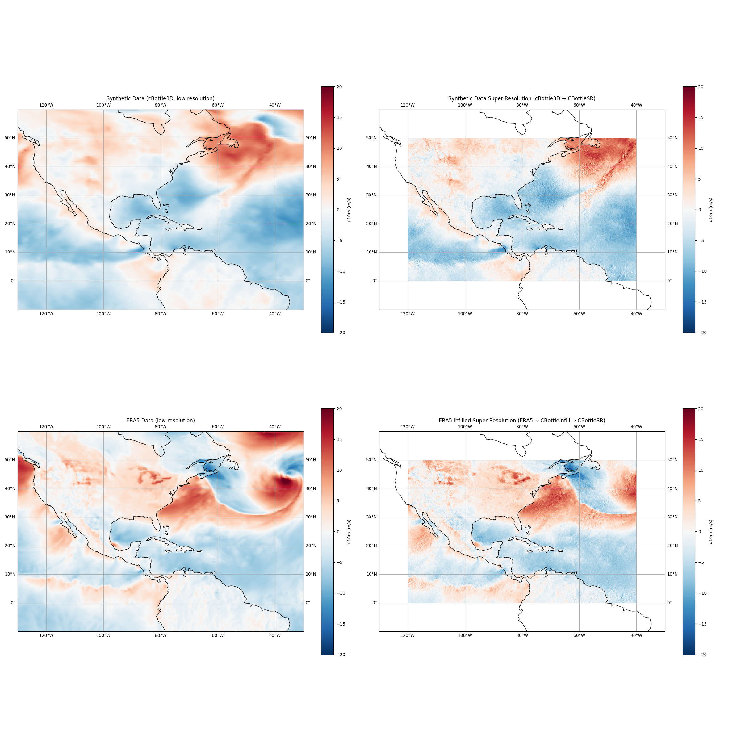
Post Processing CBottle Super Resolution Data#

Let’s visualize the super resolution results to compare the synthetic data approach with the ERA5 infilling approach. We’ll plot the total cloud liquid water (tclw) variable as an example.

import cartopy.crs as ccrs
import matplotlib.pyplot as plt

plt.close("all")

# Create projection focused on a region of interest (North Atlantic/Europe)
projection = ccrs.PlateCarree()
fig = plt.figure(figsize=(24, 24))

# Plot synthetic data
ax0 = fig.add_subplot(2, 2, 1, projection=projection)
extent = [
    super_resolution_window[1] - 10,
    super_resolution_window[3] + 10,
    super_resolution_window[0] - 10,
    super_resolution_window[2] + 10,
]
ax0.set_extent(extent, crs=ccrs.PlateCarree())
c = ax0.pcolormesh(
    synth_coords["lon"],
    synth_coords["lat"],
    synth_x[0, 0, 3, :, :].cpu().numpy(),  # u10m (variable index 3)
    transform=ccrs.PlateCarree(),
    cmap="RdBu_r",
    vmin=-20,
    vmax=20,
)
plt.colorbar(c, ax=ax0, shrink=0.6, label="u10m (m/s)")
ax0.coastlines()
ax0.gridlines(draw_labels=True)
ax0.set_title("Synthetic Data (cBottle3D, low resolution)")

# Plot the synthetic super resolution data
ax1 = fig.add_subplot(2, 2, 2, projection=projection)
ax1.set_extent(extent, crs=ccrs.PlateCarree())
c = ax1.pcolormesh(
    sr_synth_coords["lon"],
    sr_synth_coords["lat"],
    sr_synth_x[0, 0, 3, :, :].cpu().numpy(),  # u10m (variable index 3)
    transform=ccrs.PlateCarree(),
    cmap="RdBu_r",
    vmin=-20,
    vmax=20,
)
plt.colorbar(c, ax=ax1, shrink=0.6, label="u10m (m/s)")
ax1.coastlines()
ax1.gridlines(draw_labels=True)
ax1.set_title("Synthetic Data Super Resolution (cBottle3D → CBottleSR)")

# Plot the ERA5 data
ax2 = fig.add_subplot(2, 2, 3, projection=projection)
ax2.set_extent(extent, crs=ccrs.PlateCarree())
c = ax2.pcolormesh(
    era5_coords["lon"],
    era5_coords["lat"],
    era5_x[0, 0, 0, :, :].cpu().numpy(),  # u10m (variable index 0)
    transform=ccrs.PlateCarree(),
    cmap="RdBu_r",
    vmin=-20,
    vmax=20,
)
plt.colorbar(c, ax=ax2, shrink=0.6, label="u10m (m/s)")
ax2.coastlines()
ax2.gridlines(draw_labels=True)
ax2.set_title("ERA5 Data (low resolution)")

# Plot the ERA5 infilled super resolution data
ax3 = fig.add_subplot(2, 2, 4, projection=projection)
ax3.set_extent(extent, crs=ccrs.PlateCarree())
c = ax3.pcolormesh(
    sr_infill_coords["lon"],
    sr_infill_coords["lat"],
    sr_infill_x[0, 0, 3, :, :].cpu().numpy(),  # u10m (variable index 3)
    transform=ccrs.PlateCarree(),
    cmap="RdBu_r",
    vmin=-20,
    vmax=20,
)
plt.colorbar(c, ax=ax3, shrink=0.6, label="u10m (m/s)")
ax3.coastlines()
ax3.gridlines(draw_labels=True)
ax3.set_title("ERA5 Infilled Super Resolution (ERA5 → CBottleInfill → CBottleSR)")

plt.tight_layout()
plt.savefig("outputs/16_cbottle_super_resolution.jpg", dpi=150, bbox_inches="tight")

Synthetic Data (cBottle3D, low resolution), Synthetic Data Super Resolution (cBottle3D → CBottleSR), ERA5 Data (low resolution), ERA5 Infilled Super Resolution (ERA5 → CBottleInfill → CBottleSR)

Total running time of the script: (3 minutes 16.297 seconds)

Gallery generated by Sphinx-Gallery