Note
Go to the end to download the full example code.
Single Variable Perturbation Method#
Intermediate ensemble inference using a custom perturbation method.
This example will demonstrate how to run a an ensemble inference workflow with a custom perturbation method that only applies noise to a specific variable.
In this example you will learn:
How to extend an existing pertubration method
How to instantiate a built in prognostic model
Creating a data source and IO object
Running a simple built in workflow
Extend a built-in method using custom code.
Post-processing results
# /// script
# dependencies = [
#   "earth2studio[dlwp,perturbation] @ git+https://github.com/NVIDIA/earth2studio.git",
#   "matplotlib",
# ]
# ///
Set Up#
All workflows inside Earth2Studio require constructed components to be
handed to them. In this example, we will use the built in ensemble workflow
earth2studio.run.ensemble().
def ensemble(
    time: list[str] | list[datetime] | list[np.datetime64],
    nsteps: int,
    nensemble: int,
    prognostic: PrognosticModel,
    data: DataSource,
    io: IOBackend,
    perturbation: Perturbation,
    batch_size: int | None = None,
    output_coords: CoordSystem = OrderedDict({}),
    device: torch.device | None = None,
    verbose: bool = True,
) -> IOBackend:
    """Built in ensemble workflow.

    Parameters
    ----------
    time : list[str] | list[datetime] | list[np.datetime64]
        List of string, datetimes or np.datetime64
    nsteps : int
        Number of forecast steps
    nensemble : int
        Number of ensemble members to run inference for.
    prognostic : PrognosticModel
        Prognostic models
    data : DataSource
        Data source
    io : IOBackend
        IO object
    perturbation_method : Perturbation
        Method to perturb the initial condition to create an ensemble.
    batch_size: int, optional
        Number of ensemble members to run in a single batch,
        by default None.
    output_coords: CoordSystem, optional
        IO output coordinate system override, by default OrderedDict({})
    device : torch.device, optional
        Device to run inference on, by default None
    verbose : bool, optional
        Print inference progress, by default True

    Returns
    -------
    IOBackend
        Output IO object
    """
We need the following:
Prognostic Model: Use the built in DLWP model
earth2studio.models.px.DLWP.perturbation_method: Extend the Spherical Gaussian Method
earth2studio.perturbation.SphericalGaussian.Datasource: Pull data from the GFS data api
earth2studio.data.GFS.IO Backend: Save the outputs into a Zarr store
earth2studio.io.ZarrBackend.
import os

os.makedirs("outputs", exist_ok=True)
from dotenv import load_dotenv

load_dotenv()  # TODO: make common example prep function

import numpy as np
import torch

from earth2studio.data import GFS
from earth2studio.io import ZarrBackend
from earth2studio.models.px import DLWP
from earth2studio.perturbation import Perturbation, SphericalGaussian
from earth2studio.run import ensemble
from earth2studio.utils.type import CoordSystem

# Load the default model package which downloads the check point from NGC
package = DLWP.load_default_package()
model = DLWP.load_model(package)

# Create the data source
data = GFS()
The perturbation method in Running Ensemble Inference is naive because it applies the same noise amplitude to every variable. We can create a custom wrapper that only applies the perturbation method to a particular variable instead.
class ApplyToVariable:
    """Apply a perturbation to only a particular variable."""

    def __init__(self, pm: Perturbation, variable: str | list[str]):
        self.pm = pm
        if isinstance(variable, str):
            variable = [variable]
        self.variable = variable

    @torch.inference_mode()
    def __call__(
        self,
        x: torch.Tensor,
        coords: CoordSystem,
    ) -> tuple[torch.Tensor, CoordSystem]:
        # Apply perturbation
        xp, _ = self.pm(x, coords)
        # Add perturbed slice back into original tensor
        ind = np.isin(coords["variable"], self.variable)
        x[..., ind, :, :] = xp[..., ind, :, :]
        return x, coords


# Generate a new noise amplitude that specifically targets 't2m' with a 1 K noise amplitude
avsg = ApplyToVariable(SphericalGaussian(noise_amplitude=1.0), "t2m")

# Create the IO handler, store in memory
chunks = {"ensemble": 1, "time": 1, "lead_time": 1}
io = ZarrBackend(
    file_name="outputs/05_ensemble_avsg.zarr",
    chunks=chunks,
    backend_kwargs={"overwrite": True},
)
Execute the Workflow#
With all components initialized, running the workflow is a single line of Python code. Workflow will return the provided IO object back to the user, which can be used to then post process. Some have additional APIs that can be handy for post-processing or saving to file. Check the API docs for more information.
For the forecast we will predict for 10 steps (for FCN, this is 60 hours) with 8 ensemble members which will be ran in 2 batches with batch size 4.
nsteps = 10
nensemble = 8
batch_size = 4
io = ensemble(
    ["2024-01-01"],
    nsteps,
    nensemble,
    model,
    data,
    io,
    avsg,
    batch_size=batch_size,
    output_coords={"variable": np.array(["t2m", "tcwv"])},
)
2026-01-22 19:31:53.437 | INFO     | earth2studio.run:ensemble:328 - Running ensemble inference!
2026-01-22 19:31:53.437 | INFO     | earth2studio.run:ensemble:336 - Inference device: cuda

Fetching GFS data:   0%|          | 0/7 [00:00<?, ?it/s]

2026-01-22 19:31:53.520 | DEBUG    | earth2studio.data.gfs:fetch_array:382 - Fetching GFS grib file: noaa-gfs-bdp-pds/gfs.20231231/18/atmos/gfs.t18z.pgrb2.0p25.f000 420029701-1181204

Fetching GFS data:   0%|          | 0/7 [00:00<?, ?it/s]

2026-01-22 19:31:53.532 | DEBUG    | earth2studio.data.gfs:fetch_array:382 - Fetching GFS grib file: noaa-gfs-bdp-pds/gfs.20231231/18/atmos/gfs.t18z.pgrb2.0p25.f000 397402829-996456

Fetching GFS data:   0%|          | 0/7 [00:00<?, ?it/s]

2026-01-22 19:31:53.543 | DEBUG    | earth2studio.data.gfs:fetch_array:382 - Fetching GFS grib file: noaa-gfs-bdp-pds/gfs.20231231/18/atmos/gfs.t18z.pgrb2.0p25.f000 329116923-847018

Fetching GFS data:   0%|          | 0/7 [00:00<?, ?it/s]

2026-01-22 19:31:53.555 | DEBUG    | earth2studio.data.gfs:fetch_array:382 - Fetching GFS grib file: noaa-gfs-bdp-pds/gfs.20231231/18/atmos/gfs.t18z.pgrb2.0p25.f000 294691465-856457

Fetching GFS data:   0%|          | 0/7 [00:00<?, ?it/s]

2026-01-22 19:31:53.566 | DEBUG    | earth2studio.data.gfs:fetch_array:382 - Fetching GFS grib file: noaa-gfs-bdp-pds/gfs.20231231/18/atmos/gfs.t18z.pgrb2.0p25.f000 408062467-879185

Fetching GFS data:   0%|          | 0/7 [00:00<?, ?it/s]

2026-01-22 19:31:53.578 | DEBUG    | earth2studio.data.gfs:fetch_array:382 - Fetching GFS grib file: noaa-gfs-bdp-pds/gfs.20231231/18/atmos/gfs.t18z.pgrb2.0p25.f000 208052937-721817

Fetching GFS data:   0%|          | 0/7 [00:00<?, ?it/s]

2026-01-22 19:31:53.589 | DEBUG    | earth2studio.data.gfs:fetch_array:382 - Fetching GFS grib file: noaa-gfs-bdp-pds/gfs.20231231/18/atmos/gfs.t18z.pgrb2.0p25.f000 251230645-803982

Fetching GFS data:   0%|          | 0/7 [00:00<?, ?it/s]
Fetching GFS data: 100%|██████████| 7/7 [00:00<00:00, 87.36it/s]

Fetching GFS data:   0%|          | 0/7 [00:00<?, ?it/s]

2026-01-22 19:31:53.669 | DEBUG    | earth2studio.data.gfs:fetch_array:382 - Fetching GFS grib file: noaa-gfs-bdp-pds/gfs.20240101/00/atmos/gfs.t00z.pgrb2.0p25.f000 204118947-720169

Fetching GFS data:   0%|          | 0/7 [00:00<?, ?it/s]

2026-01-22 19:31:53.680 | DEBUG    | earth2studio.data.gfs:fetch_array:382 - Fetching GFS grib file: noaa-gfs-bdp-pds/gfs.20240101/00/atmos/gfs.t00z.pgrb2.0p25.f000 323956279-837771

Fetching GFS data:   0%|          | 0/7 [00:00<?, ?it/s]

2026-01-22 19:31:53.692 | DEBUG    | earth2studio.data.gfs:fetch_array:382 - Fetching GFS grib file: noaa-gfs-bdp-pds/gfs.20240101/00/atmos/gfs.t00z.pgrb2.0p25.f000 246334297-805355

Fetching GFS data:   0%|          | 0/7 [00:00<?, ?it/s]

2026-01-22 19:31:53.703 | DEBUG    | earth2studio.data.gfs:fetch_array:382 - Fetching GFS grib file: noaa-gfs-bdp-pds/gfs.20240101/00/atmos/gfs.t00z.pgrb2.0p25.f000 289307267-851916

Fetching GFS data:   0%|          | 0/7 [00:00<?, ?it/s]

2026-01-22 19:31:53.714 | DEBUG    | earth2studio.data.gfs:fetch_array:382 - Fetching GFS grib file: noaa-gfs-bdp-pds/gfs.20240101/00/atmos/gfs.t00z.pgrb2.0p25.f000 402321768-876246

Fetching GFS data:   0%|          | 0/7 [00:00<?, ?it/s]

2026-01-22 19:31:53.725 | DEBUG    | earth2studio.data.gfs:fetch_array:382 - Fetching GFS grib file: noaa-gfs-bdp-pds/gfs.20240101/00/atmos/gfs.t00z.pgrb2.0p25.f000 414179964-1179422

Fetching GFS data:   0%|          | 0/7 [00:00<?, ?it/s]

2026-01-22 19:31:53.737 | DEBUG    | earth2studio.data.gfs:fetch_array:382 - Fetching GFS grib file: noaa-gfs-bdp-pds/gfs.20240101/00/atmos/gfs.t00z.pgrb2.0p25.f000 391722290-987401

Fetching GFS data:   0%|          | 0/7 [00:00<?, ?it/s]
Fetching GFS data: 100%|██████████| 7/7 [00:00<00:00, 88.58it/s]
2026-01-22 19:31:53.777 | SUCCESS  | earth2studio.run:ensemble:358 - Fetched data from GFS
2026-01-22 19:31:53.804 | INFO     | earth2studio.run:ensemble:386 - Starting 8 Member Ensemble Inference with             2 number of batches.


Total Ensemble Batches:   0%|          | 0/2 [00:00<?, ?it/s]

Running batch 0 inference:   0%|          | 0/11 [00:00<?, ?it/s]

Running batch 0 inference:   9%|▉         | 1/11 [00:00<00:03,  3.28it/s]

Running batch 0 inference:  18%|█▊        | 2/11 [00:00<00:02,  3.10it/s]

Running batch 0 inference:  27%|██▋       | 3/11 [00:00<00:02,  3.25it/s]

Running batch 0 inference:  36%|███▋      | 4/11 [00:01<00:02,  3.27it/s]

Running batch 0 inference:  45%|████▌     | 5/11 [00:01<00:01,  3.36it/s]

Running batch 0 inference:  55%|█████▍    | 6/11 [00:01<00:01,  3.35it/s]

Running batch 0 inference:  64%|██████▎   | 7/11 [00:02<00:01,  3.40it/s]

Running batch 0 inference:  73%|███████▎  | 8/11 [00:02<00:00,  3.40it/s]

Running batch 0 inference:  82%|████████▏ | 9/11 [00:02<00:00,  3.42it/s]

Running batch 0 inference:  91%|█████████ | 10/11 [00:02<00:00,  3.38it/s]

Running batch 0 inference: 100%|██████████| 11/11 [00:03<00:00,  3.45it/s]


Total Ensemble Batches:  50%|█████     | 1/2 [00:08<00:08,  8.18s/it]

Running batch 4 inference:   0%|          | 0/11 [00:00<?, ?it/s]

Running batch 4 inference:   9%|▉         | 1/11 [00:00<00:02,  3.36it/s]

Running batch 4 inference:  18%|█▊        | 2/11 [00:00<00:02,  3.33it/s]

Running batch 4 inference:  27%|██▋       | 3/11 [00:00<00:02,  3.42it/s]

Running batch 4 inference:  36%|███▋      | 4/11 [00:01<00:02,  3.36it/s]

Running batch 4 inference:  45%|████▌     | 5/11 [00:01<00:01,  3.42it/s]

Running batch 4 inference:  55%|█████▍    | 6/11 [00:01<00:01,  3.39it/s]

Running batch 4 inference:  64%|██████▎   | 7/11 [00:02<00:01,  3.42it/s]

Running batch 4 inference:  73%|███████▎  | 8/11 [00:02<00:00,  3.40it/s]

Running batch 4 inference:  82%|████████▏ | 9/11 [00:02<00:00,  3.44it/s]

Running batch 4 inference:  91%|█████████ | 10/11 [00:02<00:00,  3.41it/s]

Running batch 4 inference: 100%|██████████| 11/11 [00:03<00:00,  3.43it/s]


Total Ensemble Batches: 100%|██████████| 2/2 [00:16<00:00,  8.16s/it]
Total Ensemble Batches: 100%|██████████| 2/2 [00:16<00:00,  8.16s/it]
2026-01-22 19:32:10.134 | SUCCESS  | earth2studio.run:ensemble:438 - Inference complete
Post Processing#
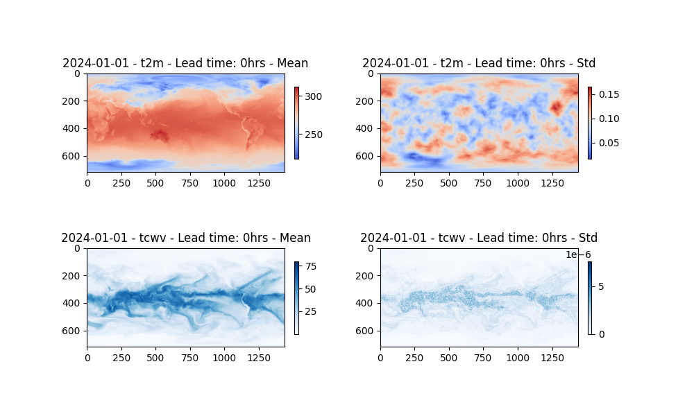
The last step is to post process our results. Lets plot both the perturbed t2m field and also the unperturbed tcwv field. First to confirm the perturbation method works as expect, the initial state is plotted.
Notice that the Zarr IO function has additional APIs to interact with the stored data.
import matplotlib.pyplot as plt

forecast = "2024-01-01"


def plot_(axi, data, title, cmap):
    """Simple plot util function"""
    im = axi.imshow(data, cmap=cmap)
    plt.colorbar(im, ax=axi, shrink=0.5, pad=0.04)
    axi.set_title(title)


step = 0  # lead time = 24 hrs
plt.close("all")

# Create a figure and axes with the specified projection
fig, ax = plt.subplots(nrows=2, ncols=2, figsize=(10, 6))
plot_(
    ax[0, 0],
    np.mean(io["t2m"][:, 0, step], axis=0),
    f"{forecast} - t2m - Lead time: {6*step}hrs - Mean",
    "coolwarm",
)
plot_(
    ax[0, 1],
    np.std(io["t2m"][:, 0, step], axis=0),
    f"{forecast} - t2m - Lead time: {6*step}hrs - Std",
    "coolwarm",
)
plot_(
    ax[1, 0],
    np.mean(io["tcwv"][:, 0, step], axis=0),
    f"{forecast} - tcwv - Lead time: {6*step}hrs - Mean",
    "Blues",
)
plot_(
    ax[1, 1],
    np.std(io["tcwv"][:, 0, step], axis=0),
    f"{forecast} - tcwv - Lead time: {6*step}hrs - Std",
    "Blues",
)

plt.savefig(f"outputs/05_{forecast}_{step}_ensemble.jpg")
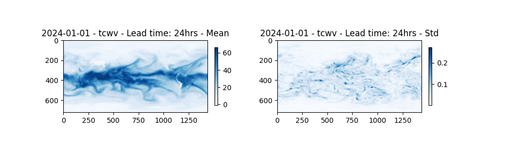
Due to the intrinsic coupling between all fields, we should expect all variables to have some uncertainty for later lead times. Here the total column water vapor is plotted at a lead time of 24 hours, note the variance in the members despite just perturbing the temperature field.
step = 4  # lead time = 24 hrs
plt.close("all")

# Create a figure and axes with the specified projection
fig, ax = plt.subplots(nrows=1, ncols=2, figsize=(10, 3))
plot_(
    ax[0],
    np.mean(io["tcwv"][:, 0, step], axis=0),
    f"{forecast} - tcwv - Lead time: {6*step}hrs - Mean",
    "Blues",
)
plot_(
    ax[1],
    np.std(io["tcwv"][:, 0, step], axis=0),
    f"{forecast} - tcwv - Lead time: {6*step}hrs - Std",
    "Blues",
)

plt.savefig(f"outputs/05_{forecast}_{step}_ensemble.jpg")
Total running time of the script: (0 minutes 20.216 seconds)