Velocity Verlet Dynamics with Lennard-Jones Potential

This example demonstrates GPU-accelerated molecular dynamics using the Velocity Verlet integrator with a Lennard-Jones (LJ) potential.

We simulate argon in the NVE ensemble (no thermostat) to demonstrate:

1. Building an FCC lattice system

2. Computing neighbor lists with periodic boundaries

3. Using the LJ potential for energy and forces

4. Running Velocity Verlet dynamics

5. Monitoring energy conservation and basic stability diagnostics

Notes

Velocity Verlet is stable and time-reversible, but for LJ systems it is still sensitive to: - timestep size, - neighbor list rebuild logic, - force discontinuities at the cutoff (consider using switch_width > 0).

Imports

from __future__ import annotations

import matplotlib.pyplot as plt
import numpy as np
import warp as wp
from _dynamics_utils import (
    DEFAULT_CUTOFF,
    DEFAULT_SKIN,
    EPSILON_AR,
    SIGMA_AR,
    MDSystem,
    create_fcc_argon,
    run_velocity_verlet,
)

System setup

print("=" * 95)
print("VELOCITY VERLET DYNAMICS WITH LENNARD-JONES POTENTIAL (NVE)")
print("=" * 95)
print()

device = "cuda:0" if wp.is_cuda_available() else "cpu"
print(f"Using device: {device}")

print("\n--- Creating FCC Argon System ---")
positions, cell = create_fcc_argon(num_unit_cells=4, a=5.26)  # 256 atoms
print(f"Created {len(positions)} atoms in {cell[0, 0]:.2f} ų box")

print("\n--- Initializing MD System ---")
system = MDSystem(
    positions=positions,
    cell=cell,
    epsilon=EPSILON_AR,
    sigma=SIGMA_AR,
    cutoff=DEFAULT_CUTOFF,
    skin=DEFAULT_SKIN,
    # NVE can benefit from smooth cutoffs; keep hard cutoff by default for now.
    switch_width=0.0,
    device=device,
    dtype=np.float64,
)

print("\n--- Setting Initial Temperature ---")
system.initialize_temperature(temperature=94.4, seed=42)

===============================================================================================
VELOCITY VERLET DYNAMICS WITH LENNARD-JONES POTENTIAL (NVE)
===============================================================================================

Using device: cuda:0

--- Creating FCC Argon System ---
Created 256 atoms in 21.04 ų box

--- Initializing MD System ---
Initialized MD system with 256 atoms
  Cell: 21.04 x 21.04 x 21.04 Å
  Cutoff: 8.50 Å (+ 0.50 Å skin)
  LJ: ε = 0.0104 eV, σ = 3.40 Å
  Device: cuda:0, dtype: <class 'numpy.float64'>
  Units: x [Å], t [fs], E [eV], m [eV·fs²/Ų] (from amu), v [Å/fs]

--- Setting Initial Temperature ---
Initialized velocities: target=94.4 K, actual=90.4 K

Velocity Verlet (NVE)

print("\n--- NVE Run (3000 steps) ---")
stats = run_velocity_verlet(
    system=system,
    num_steps=3000,
    dt_fs=1.0,
    log_interval=200,
)

--- NVE Run (3000 steps) ---

Running 3000 Velocity Verlet steps (NVE)
  dt = 1.000 fs
===============================================================================================
    Step      KE (eV)      PE (eV)   Total (eV)      T (K)  Neighbors  min r (Å)     max|F|
===============================================================================================
       0       2.9787     -21.5621     -18.5833      90.37       9984      3.713  2.313e-03
     200       1.2443     -19.7214     -18.4771      37.75      10304      3.324  1.422e-01
     400       1.5604     -20.0374     -18.4771      47.34      10256      3.313  1.771e-01
     600       1.3336     -19.8084     -18.4749      40.46      10279      3.344  1.640e-01
     800       1.5552     -20.0421     -18.4869      47.18      10253      3.239  1.964e-01
    1000       1.5486     -20.0457     -18.4971      46.98      10265      3.316  1.433e-01
    1200       1.5071     -19.9964     -18.4893      45.72      10266      3.322  1.814e-01
    1400       1.4764     -19.9599     -18.4835      44.79      10275      3.253  1.971e-01
    1600       1.5812     -20.0671     -18.4859      47.97      10245      3.318  1.719e-01
    1800       1.5937     -20.0755     -18.4818      48.35      10269      3.317  1.582e-01
    2000       1.5902     -20.0884     -18.4983      48.24      10268      3.351  1.498e-01
    2200       1.4885     -19.9817     -18.4932      45.16      10260      3.302  1.611e-01
    2400       1.4969     -19.9773     -18.4805      45.41      10257      3.331  1.949e-01
    2600       1.4802     -19.9617     -18.4815      44.91      10267      3.296  1.753e-01
    2800       1.4200     -19.9046     -18.4845      43.08      10257      3.292  1.663e-01
    2999       1.5927     -20.0865     -18.4939      48.32      10252      3.272  1.715e-01

Analysis

print("\n--- Analysis ---")
temps = np.array([s.temperature for s in stats])
total_energies = np.array([s.total_energy for s in stats])
steps = np.array([s.step for s in stats])

e0 = total_energies[0]
drift = total_energies - e0

print(f"  Mean Temperature:    {temps.mean():.2f} ± {temps.std():.2f} K")
print(f"  Mean Total Energy:   {total_energies.mean():.4f} eV")
print(f"  Energy Fluctuation:  {total_energies.std():.4f} eV")
print(
    f"  Energy Drift (last): {drift[-1]:.6f} eV  (relative: {drift[-1] / e0 * 100:.3e}%)"
)

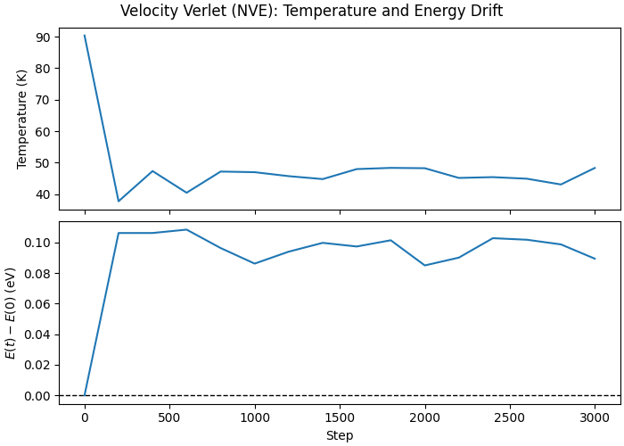
fig, ax = plt.subplots(2, 1, figsize=(7.0, 5.0), sharex=True, constrained_layout=True)
ax[0].plot(steps, temps, lw=1.5)
ax[0].set_ylabel("Temperature (K)")
ax[1].plot(steps, drift, lw=1.5)
ax[1].axhline(0.0, color="k", ls="--", lw=1.0)
ax[1].set_xlabel("Step")
ax[1].set_ylabel(r"$E(t) - E(0)$ (eV)")
fig.suptitle("Velocity Verlet (NVE): Temperature and Energy Drift")

print("\n" + "=" * 95)
print("SIMULATION COMPLETE")
print("=" * 95)

--- Analysis ---
  Mean Temperature:    48.25 ± 11.24 K
  Mean Total Energy:   -18.4918 eV
  Energy Fluctuation:  0.0246 eV
  Energy Drift (last): 0.089460 eV  (relative: -4.814e-01%)

===============================================================================================
SIMULATION COMPLETE
===============================================================================================