NPT Dynamics (MTK + Nosé-Hoover Chain) with Lennard-Jones Potential

This example demonstrates isothermal-isobaric (NPT) dynamics using the Martyna-Tobias-Klein (MTK) barostat coupled with a Nosé-Hoover chain (NHC) thermostat, driven by the Lennard-Jones (LJ) potential.

from __future__ import annotations

import matplotlib.pyplot as plt
import numpy as np
import warp as wp
from _dynamics_utils import (
    DEFAULT_CUTOFF,
    DEFAULT_SKIN,
    EPSILON_AR,
    SIGMA_AR,
    MDSystem,
    create_fcc_argon,
    pressure_atm_to_ev_per_a3,
    run_npt_mtk,
)

print("=" * 95)
print("NPT (MTK + NHC) DYNAMICS WITH LENNARD-JONES POTENTIAL")
print("=" * 95)
print()

device = "cuda:0" if wp.is_cuda_available() else "cpu"
print(f"Using device: {device}")

print("\n--- Creating FCC Argon System ---")
positions, cell = create_fcc_argon(num_unit_cells=4, a=5.26)  # 256 atoms
print(f"Created {len(positions)} atoms in {cell[0, 0]:.2f} ų box")

print("\n--- Initializing MD System ---")
system = MDSystem(
    positions=positions,
    cell=cell,
    epsilon=EPSILON_AR,
    sigma=SIGMA_AR,
    cutoff=DEFAULT_CUTOFF,
    skin=DEFAULT_SKIN,
    switch_width=0.0,
    device=device,
    dtype=np.float64,
)

print("\n--- Setting Initial Temperature ---")
system.initialize_temperature(temperature=94.4, seed=42)

===============================================================================================
NPT (MTK + NHC) DYNAMICS WITH LENNARD-JONES POTENTIAL
===============================================================================================

Using device: cuda:0

--- Creating FCC Argon System ---
Created 256 atoms in 21.04 ų box

--- Initializing MD System ---
Initialized MD system with 256 atoms
  Cell: 21.04 x 21.04 x 21.04 Å
  Cutoff: 8.50 Å (+ 0.50 Å skin)
  LJ: ε = 0.0104 eV, σ = 3.40 Å
  Device: cuda:0, dtype: <class 'numpy.float64'>
  Units: x [Å], t [fs], E [eV], m [eV·fs²/Ų] (from amu), v [Å/fs]

--- Setting Initial Temperature ---
Initialized velocities: target=94.4 K, actual=90.4 K

print("\n--- NPT Run (3000 steps) ---")
print(f"Pressure units sanity: 1 atm = {pressure_atm_to_ev_per_a3(1.0):.6e} eV/ų")
stats = run_npt_mtk(
    system=system,
    num_steps=3000,
    dt_fs=1.0,
    target_temperature_K=94.4,
    target_pressure_atm=1.0,
    tdamp_fs=500.0,
    pdamp_fs=5000.0,
    chain_length=3,
    log_interval=200,
)

--- NPT Run (3000 steps) ---
Pressure units sanity: 1 atm = 6.324209e-07 eV/ų

Running 3000 NPT (MTK) steps at T=94.4 K, P=1.000 atm
  dt = 1.000 fs, tdamp = 500.0 fs, pdamp = 5000.0 fs, chain_length = 3
========================================================================================================================
    Step      KE (eV)      PE (eV)   Total (eV)      T (K)    P (atm)    V (Å^3)  Neighbors  min r (Å)     max|F|
========================================================================================================================
       0       2.9787     -21.5621     -18.5833      90.37    483.900    9314.02       9984      3.713  2.313e-03
     200       1.2863     -19.7064     -18.4201      39.02   1892.990    9315.31      10305      3.322  1.434e-01
     400       1.6828     -19.9228     -18.2400      51.05   1730.950    9320.49      10255      3.299  1.882e-01
     600       1.5355     -19.5738     -18.0382      46.59   1987.243    9329.58      10281      3.325  1.769e-01
     800       1.9030     -19.7130     -17.8100      57.73   1854.898    9343.17      10253      3.221  2.158e-01
    1000       2.0381     -19.5912     -17.5531      61.83   1927.512    9361.65      10266      3.264  1.809e-01
    1200       2.1232     -19.3932     -17.2700      64.42   2017.448    9385.47      10255      3.271  2.251e-01
    1400       2.2290     -19.2150     -16.9860      67.63   2080.926    9415.26      10238      3.161  3.116e-01
    1600       2.4932     -19.2021     -16.7090      75.64   2009.581    9451.65      10206      3.236  2.207e-01
    1800       2.6645     -19.0812     -16.4167      80.84   1990.881    9494.97      10190      3.175  2.831e-01
    2000       2.8024     -18.9681     -16.1657      85.02   1964.547    9545.52      10196      3.245  1.976e-01
    2200       2.8151     -18.7167     -15.9016      85.41   1992.528    9603.67      10170      3.205  2.329e-01
    2400       2.8787     -18.5592     -15.6805      87.33   1935.112    9669.43      10087      3.221  2.472e-01
    2600       3.0736     -18.5307     -15.4572      93.25   1766.366    9743.08      10041      3.223  2.592e-01
    2800       2.9836     -18.2642     -15.2806      90.52   1753.716    9824.49       9969      3.233  2.417e-01
    2999       3.1615     -18.2752     -15.1137      95.92   1519.791    9913.24       9970      3.189  2.508e-01

print("\n--- Analysis ---")
temps = np.array([s.temperature for s in stats])
pressures_atm = np.array([s.pressure for s in stats])
volumes = np.array([s.volume for s in stats])
steps = np.array([s.step for s in stats])

print(f"  Mean Temperature: {temps.mean():.2f} ± {temps.std():.2f} K")
print("  Target Temperature: 94.4 K")
print()
print(f"  Mean Pressure:    {pressures_atm.mean():.3f} ± {pressures_atm.std():.3f} atm")
print("  Target Pressure:  1.0 atm")
print()
print(f"  Mean Volume:      {volumes.mean():.2f} ± {volumes.std():.2f} ų")

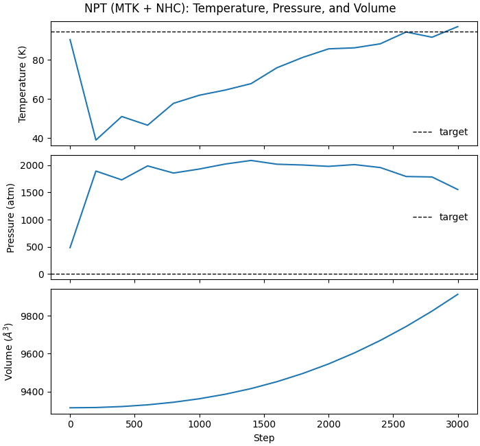
fig, ax = plt.subplots(3, 1, figsize=(7.0, 6.5), sharex=True, constrained_layout=True)
ax[0].plot(steps, temps, lw=1.5)
ax[0].axhline(94.4, color="k", ls="--", lw=1.0, label="target")
ax[0].set_ylabel("Temperature (K)")
ax[0].legend(frameon=False, loc="best")
ax[1].plot(steps, pressures_atm, lw=1.5)
ax[1].axhline(1.0, color="k", ls="--", lw=1.0, label="target")
ax[1].set_ylabel("Pressure (atm)")
ax[1].legend(frameon=False, loc="best")
ax[2].plot(steps, volumes, lw=1.5)
ax[2].set_xlabel("Step")
ax[2].set_ylabel(r"Volume ($\AA^3$)")
fig.suptitle("NPT (MTK + NHC): Temperature, Pressure, and Volume")

print("\n" + "=" * 95)
print("SIMULATION COMPLETE")
print("=" * 95)

--- Analysis ---
  Mean Temperature: 73.29 ± 17.52 K
  Target Temperature: 94.4 K

  Mean Pressure:    1806.774 ± 368.263 atm
  Target Pressure:  1.0 atm

  Mean Volume:      9501.94 ± 189.24 ų

===============================================================================================
SIMULATION COMPLETE
===============================================================================================