import numpy as np

rng = np.random.default_rng(2026)
sample_rate = 1024.0  # Hz
a = rng.normal(size=8192).astype(np.float32)
b = np.zeros_like(a)
b[7:] = a[:-7]  # b hears a 7 samples late
b += 0.5 * rng.normal(size=b.size).astype(np.float32)13 Correlate signals
xBeam (cuphoton.xbeam) correlates sampled signals. Two sensors that record one source, such as two microphones or two radio telescopes, share a delayed copy of it. xBeam measures how much the recordings share and at what delay, frequency by frequency. correlate_series cuts each signal into windows, takes the fast Fourier transform (FFT) of each window, multiplies one transform by the conjugate of the other and averages. It returns cross-spectra, lag correlations, or both. For radio astronomy, cuphoton xbeam correlate turns VDIF recordings into visibilities (Section 13.11).
You need:
- cuPhoton with the CPU profile (Chapter 1). xBeam needs no extra on the CPU.
- The
gpuprofile and an NVIDIA GPU for the GPU paths. - Two or more uniformly sampled signals on one time grid, or the sample pair below.
NoteSample data
This page runs on a small synthetic pair. The printed values only demonstrate the API.
13.1 Make two signals with a known delay
Signal b below is a copy of signal a that arrives 7 samples later, plus noise of its own:
13.2 Wrap the signals in a source
A source names each signal and holds the shared sample grid. ArraySource wraps NumPy or CuPy vectors:
from cuphoton.xbeam import ArraySource

source = ArraySource({"a": a, "b": b}, sample_rate_hz=sample_rate)
print(source.signal_ids, source.sample_count, source.sample_rate_hz)
('a', 'b') 8192 1024.0All signals in a source share one length, sample rate and time origin. Resample or correct clocks before you correlate. Hdf5Source reads signals from an HDF5 file instead (Section 13.6).
13.3 Correlate the pair
A CorrelationSpec names the pairs to correlate and sets how to cut the signals into windows (Section 13.8). correlate_series yields one result per group of windows_per_result windows:
from cuphoton.xbeam import CorrelationSpec, correlate_series

spec = CorrelationSpec(pairs=(("a", "b"),), window_samples=1024, windows_per_result=4, output="both")
results = list(correlate_series(source, spec))
for r in results:
    print(f"result {r.result_index}: samples {r.sample_start} to {r.sample_stop}, "
          f"spectrum {r.spectrum.shape}, lag {r.lag.shape}")
result 0: samples 0 to 4096, spectrum (1, 2048), lag (1, 2047)
result 1: samples 4096 to 8192, spectrum (1, 2048), lag (1, 2047)The 8,192 samples make eight windows of 1,024, and therefore two results of four windows. Each array has one row per pair. A SeriesResult holds these fields as host NumPy arrays:
| Field | Holds |
|---|---|
spectrum, frequencies_hz |
the cross-spectrum per pair, and its frequencies in standard FFT order |
lag, lag_samples |
the lag correlation per pair, and its lags in samples |
lag_valid_samples |
the valid sample pairs at each lag, summed over the windows |
simultaneous_valid_samples, contributing_windows, valid |
coverage counts per pair, and whether the pair had any valid data |
result_index, sample_start, sample_stop, window_starts |
the result’s position in the series |
Products are raw sums averaged over the windows. xBeam applies no taper, mean removal or normalization. Add the pair ("a", "a") for an autocorrelation to normalize by.
13.4 Read the delay from the lag correlation
The lag correlation is R(k) = sum_n a[n] * conj(b[n + k]). It peaks at the delay. A positive lag means the second signal of the pair arrives later:
for r in results:
    peak = r.lag_samples[np.argmax(np.abs(r.lag[0]))]
    print(f"result {r.result_index}: b arrives {peak} samples ({1e3 * peak / r.sample_rate_hz:.2f} ms) after a")
result 0: b arrives 7 samples (6.84 ms) after a
result 1: b arrives 7 samples (6.84 ms) after aDivide lag_samples by sample_rate_hz for seconds. The peak gives a whole number of samples.
13.5 Read the delay from the cross-spectrum
The cross-spectrum is FFT(a) * conj(FFT(b)). When b arrives τ seconds late, the phase at frequency f is 2πfτ. The slope of the phase against frequency therefore measures the delay, including fractions of a sample. Average the results, then fit a line to the unwrapped phase at positive frequencies:
spectrum = np.mean([r.spectrum[0] for r in results], axis=0)
freq = results[0].frequencies_hz
positive = freq > 0
phase = np.unwrap(np.angle(spectrum[positive]))
slope = np.polyfit(freq[positive], phase, 1)[0]  # radians per Hz
print(f"phase slope: {slope / (2 * np.pi) * sample_rate:.2f} samples")
phase slope: 7.00 samplesFigure 13.1 shows both readings.
Plotting code
import matplotlib.pyplot as plt

near = np.abs(results[0].lag_samples) <= 20
fig, (ax_lag, ax_phase) = plt.subplots(1, 2, figsize=(6.5, 2.6))
ax_lag.bar(results[0].lag_samples[near], results[0].lag[0, near].real, color="#2A78D6", width=0.8)
ax_lag.set_xlabel("Lag (samples)")
ax_lag.set_ylabel("Lag correlation")
ax_phase.plot(freq[positive], phase, color="#2A78D6", lw=0.8)
line = np.polyval(np.polyfit(freq[positive], phase, 1), freq[positive])
ax_phase.plot(freq[positive], line, "--", color="#EB6834", lw=1.4)
ax_phase.set_xlabel("Frequency (Hz)")
ax_phase.set_ylabel("Phase (rad)")
fig.text(1, 1, "Synthetic data, for demonstration only", ha="right", va="bottom",
         fontsize=7, style="italic", color="0.4", transform=fig.transFigure)
fig.tight_layout()
plt.show()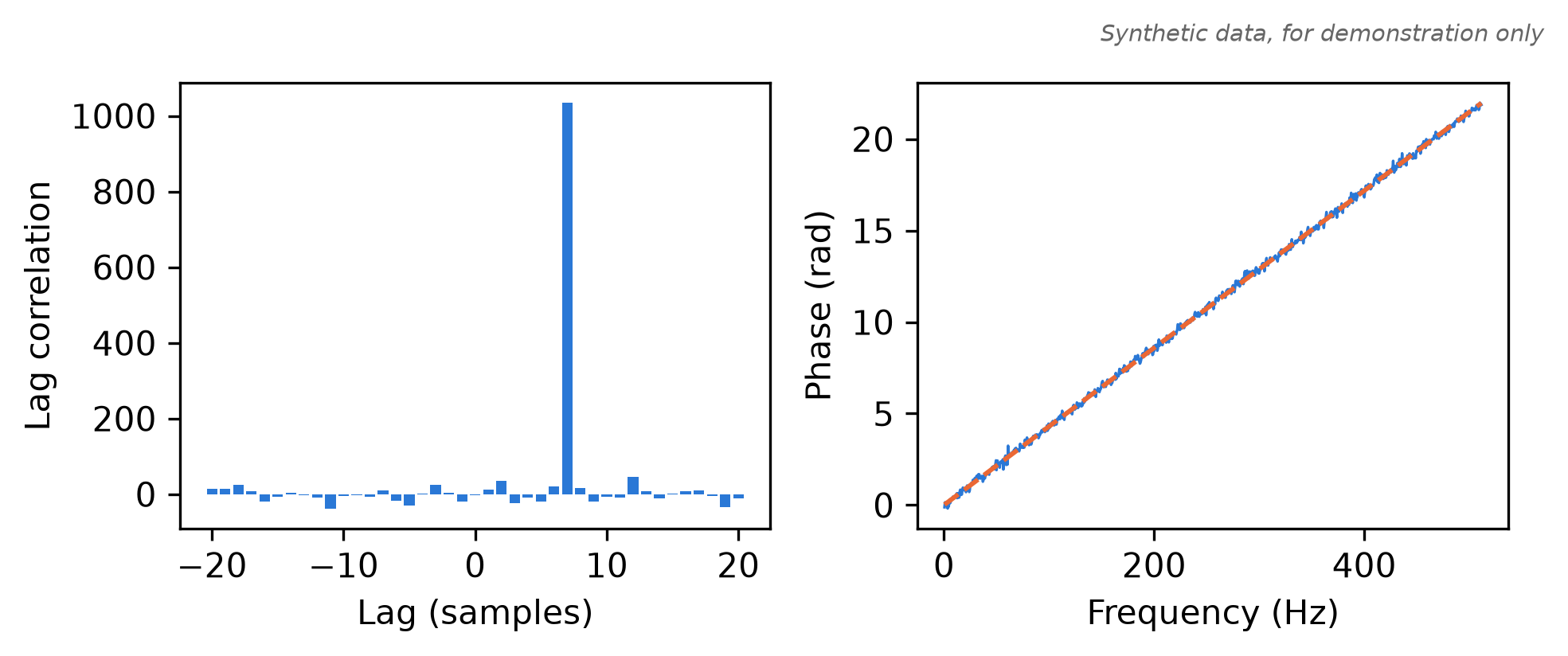
b matches a. Right: the unwrapped phase of the averaged cross-spectrum (blue) and the fitted line (dashed orange). Its slope is 2π times the delay in seconds. Synthetic data, for demonstration only.
13.6 Correlate signals stored in HDF5
Hdf5Source reads each signal from a one-dimensional dataset in an HDF5 file (Hierarchical Data Format 5, a format for named arrays). Each dataset has scalar sample_rate_hz and origin_seconds attributes. Write the sample pair to signals.h5:
import h5py

with h5py.File("signals.h5", "w") as h5:
    for name, samples in (("a", a), ("b", b)):
        dataset = h5.create_dataset(f"signals/{name}", data=samples)
        dataset.attrs["sample_rate_hz"] = sample_rate
        dataset.attrs["origin_seconds"] = 0.0
Hdf5Source reads bounded slices, not the whole file. Use it as a context manager and consume the results inside the with block:
from cuphoton.xbeam import Hdf5Source

with Hdf5Source("signals.h5", {"a": "/signals/a", "b": "/signals/b"}) as file_source:
    peaks = [int(r.lag_samples[np.argmax(np.abs(r.lag[0]))]) for r in correlate_series(file_source, spec)]
print(peaks)
[7, 7]By default, the source reads the next batch of windows on a background thread. Set prefetch_batches=0 in the spec for synchronous reads.
13.7 Shard a long series
To split a long recording among independent tasks, give every task the same spec with a common shard_count and its own shard_index. plan_series_shards shows which results and samples each shard covers:
from cuphoton.xbeam import plan_series_shards

sharded = CorrelationSpec(pairs=(("a", "b"),), window_samples=1024, windows_per_result=4,
                          output="lag", shard_count=2, shard_index=1)
for shard in plan_series_shards(source.sample_count, sharded):
    print(shard)
print("shard 1 yields results", [r.result_index for r in correlate_series(source, sharded)])
SeriesShard(index=0, first_result=0, stop_result=1, sample_start=0, sample_stop=4096)
SeriesShard(index=1, first_result=1, stop_result=2, sample_start=4096, sample_stop=8192)
shard 1 yields results [1]Each shard keeps the global result_index. Write each shard to its own output and combine the results by that index. Do not average shard outputs. With overlapping windows (hop_samples below window_samples), shards read a few shared samples and still emit each result once.
13.8 Options
CorrelationSpec takes these fields:
| Option | Default | Effect |
|---|---|---|
pairs |
required | Signal-name pairs to correlate. ("a", "a") gives an autocorrelation. |
window_samples |
required | Samples per FFT window |
hop_samples |
None |
Step between window starts. None uses window_samples. |
windows_per_result |
1 |
Windows averaged into one result |
output |
"spectrum" |
"spectrum", "lag" or "both" |
lag_mode |
"linear" |
"linear" zero-pads each window. Lags run from -(window_samples - 1) to window_samples - 1. "circular" uses a window_samples-point FFT, and the correlation wraps. |
precision |
None |
"float32" or "float64". None keeps the input float precision and uses float64 for integers. |
batch_windows |
16 |
Windows per transform batch. Bounds working memory. |
backend |
"numpy" |
"cupy" runs the transforms and products on the GPU |
shard_index, shard_count |
0, 1 |
This task’s shard, and the number of shards |
prefetch_batches |
1 |
1 reads the next HDF5 batch ahead, 0 reads synchronously |
To mark gaps, pass Boolean validity vectors to the source, such as ArraySource(..., validity={"b": mask}). xBeam sets invalid samples to zero before the transforms and reports the coverage counts. Where lag_valid_samples is above zero, the mean over valid sample pairs is len(window_starts) * lag / lag_valid_samples.
13.9 On a GPU
With the gpu profile, or the smaller io extra, set backend="cupy" in the spec. The transforms and products run on the GPU, and the results are host NumPy arrays:
import cupy as cp

gpu_source = ArraySource({"a": cp.asarray(a), "b": cp.asarray(b)}, sample_rate_hz=sample_rate)
gpu_spec = CorrelationSpec(pairs=(("a", "b"),), window_samples=1024, windows_per_result=4,
                           output="both", backend="cupy")
gpu_results = list(correlate_series(gpu_source, gpu_spec))
Add result_location="device" to the spec to keep the products on the GPU as CuPy arrays. Before consuming them on a CUDA stream, call result.wait(stream) to order that stream after the result’s work. result.to_host() waits and copies one result to the host.
For HDF5 input, Hdf5Source reads slices on the host and uploads them asynchronously. With io_backend="cufile", it reads them into GPU memory through GPUDirect Storage. That path needs a working GDS installation and supported filesystem, plus the HDF5 sec2 driver and contiguous, uncompressed datasets with native numeric types. Every signal and validity dataset must belong to the opened file, with an offset and byte size divisible by 4096.
The sample file above uses ordinary HDF5 allocation and is not guaranteed to meet those alignment requirements. To create an aligned version, use h5py.File("signals.h5", "w", alignment_threshold=1, alignment_interval=4096) in its creation block and choose array lengths whose byte sizes are divisible by 4096. The sample’s 8192-element float32 arrays meet the size requirement. Unsupported layouts raise an error instead of switching to POSIX reads.
On the command line, add --backend cupy, and set io_backend at the top level of the JSON file. --upload-workers caps the input workers, at auto or 1 to 16. Select one GPU per shard task through CUDA_VISIBLE_DEVICES.
13.10 Command line
correlate-series reads a JSON file. Its correlation object holds the CorrelationSpec fields except backend, which the command sets. The input path is relative to the JSON file:
import json
from pathlib import Path

config = {
    "input": "signals.h5",
    "datasets": {"a": "/signals/a", "b": "/signals/b"},
    "correlation": {"pairs": [["a", "b"]], "window_samples": 1024, "windows_per_result": 4, "output": "both"},
}
Path("series.json").write_text(json.dumps(config, indent=2))258Run it. The command prints nothing on success and never overwrites an existing output file:
cuphoton xbeam correlate-series series.json --output results.h5 --backend numpyThe file stores each result under /results/<result_index>, with arrays named after the SeriesResult fields:
with h5py.File("results.h5") as h5:
    print(h5.attrs["schema"], "complete:", h5.attrs["complete"], "results:", list(h5["results"]))
    first = h5["results/0"]
    print(first.attrs["pairs_json"], first["lag"].shape, first["spectrum"].shape)
cuphoton-series-v1 complete: True results: ['0', '1']
[["a", "b"]] (1, 2047) (1, 2048)An interrupted write leaves complete false. For sharded runs, put shard_count and shard_index in the correlation object and give each task its own JSON file and output.
13.11 Correlate radio recordings
The radio path correlates recordings from radio telescopes (stations) and writes visibilities, the averaged cross-spectra from which interferometry makes images. It needs two inputs:
- A job, as a normalized JSON file or as supported
.inputmetadata from the DiFX software correlator. The job lists the stations, clocks, frequency bands, baselines and delay models. - The recordings, as VDIF files (the data format of very long baseline interferometry). A VDIF file holds frames of packed samples behind headers. xBeam reads file-backed, two-bit, non-legacy VDIF with oversampling and decimation factors of one.
Replace job.json, AA.vdif and BB.vdif with your files. This page does not run these commands:
# Check a recording's frame headers
cuphoton xbeam inspect-vdif AA.vdif --json

# Index each recording once, with POSIX reads
cuphoton xbeam build-vdif-sidecar AA.vdif BB.vdif --index-dir sidecars --backend posix

# Correlate on the CPU into a new directory
cuphoton xbeam correlate job.json --output visibilities --backend numpy --index-dir sidecars
build-vdif-sidecar writes a header index (a sidecar, .vdix) for each recording. Its --backend selects the read path and defaults to cufile, which needs GPUDirect Storage. Correlation does not build missing sidecars. Without one, pass --assume-ordered only for recordings you checked are in time order. For correlate, --backend selects NumPy or CuPy and --vdif-io the GPU read path.
The output directory must be new. It holds the native xbeam-v1 format (metadata.jsonl and spectra.c64), or the DiFX SWIN format if the job selects it, plus ingest-manifest.json. Each record holds a spectrum, its time, weight, station pair and baseline coordinates. From Python, correlate(load_job("job.json"), backend="numpy", index_dir="sidecars") yields the same records. read_xbeam_v1 in cuphoton.xbeam.adapters.radio.output reads a native output directory.
On a GPU, add --backend cupy. --vdif-io cufile reads through GPUDirect Storage. --devices splits a scan window into contiguous time shards across the listed devices:
cuphoton xbeam correlate job.json --output visibilities-gpu --backend cupy --index-dir sidecars \
  --scan SCAN --first-integration 0 --integration-count 100 --devices 0,1
Time sharding needs --scan, --first-integration and --integration-count together. To run shards under an external scheduler, give each task that same parent scan window and --shard-count, its own --shard-index, and a separate output directory. Assemble the complete set of parts with merge-shards.
13.12 Troubleshooting
- No results. Only complete groups of
windows_per_resultwindows produce results. Use a shorter window or fewer windows per result. nonfinite valid samples in 'b'. A sample marked valid is NaN or infinite. Mark it invalid with avalidityvector.requested pair contains an unavailable signal. A name inpairsis not in the source.signals do not share a common sample grid. The HDF5 datasets differ insample_rate_hzororigin_seconds. Resample them first.File existsfromcorrelate-series. The command never overwrites. Choose a new--output.- The lag peak is at the wrong place. The delay can exceed the window. Linear mode covers lags up to
window_samples - 1. Use longer windows.
13.13 Next steps
- Time-series reference, with the HDF5 layout and conventions: time-series correlation.
- Radio jobs and outputs: the xBeam guide, the data contract, sidecars and compatibility profiles.
- Run shards on many GPUs or nodes: Chapter 14.
- Fit damped oscillations in one signal instead: Chapter 12.