This tutorial takes two images of the same sky and finds what changed between them. You read the images, put one on the other’s pixel grid, match their blur, subtract, find the candidates and measure them. It uses four modules: Core reads the files, xRep aligns, xPois subtracts and detects, and xFit measures. The example runs on a CPU; its runtime depends on the host.
You need: cuPhoton installed with the CPU profile (Chapter 1). No GPU and no data files: the first step makes a small sample pair.
NoteSample data
This page runs on a small synthetic pair. The printed values only demonstrate the API.
2.1 Make a sample pair
The block below writes sample/reference.fits and sample/target.fits. They are two synthetic star fields of the same patch of sky. The reference is sharper and deeper. The target is rotated by 3 degrees, has slightly larger pixels, more blur and a brighter sky. It also holds one new source and one star that became three times brighter. You do not need to read the code. Expand it to copy it.
Create the sample pair (NumPy and Astropy only)
# Writes sample/reference.fits and sample/target.fits: two synthetic star fields# of the same sky on different pixel grids, with different blur and sky level.# The target also holds one new source and one star three times brighter.# Noise is independent Gaussian noise with variance expected_image / gain;# this teaching sample has no read noise, saturation, or detector artifacts.from pathlib import Pathimport numpy as npfrom astropy.io import fitsfrom astropy.wcs import WCSrng = np.random.default_rng(7)def make_wcs(shape, scale_arcsec, rotation_deg, crpix_shift): w = WCS(naxis=2) w.wcs.ctype = ["RA---TAN", "DEC--TAN"] w.wcs.crval = [150.0, 2.0] w.wcs.crpix = [shape[1] /2+ crpix_shift[0], shape[0] /2+ crpix_shift[1]] c, s = np.cos(np.radians(rotation_deg)), np.sin(np.radians(rotation_deg)) w.wcs.cd = scale_arcsec /3600* np.array([[-c, s], [s, c]])return wdef render(shape, wcs, ra, dec, flux, sigma, sky, gain): x, y = wcs.world_to_pixel_values(ra, dec) yy, xx = np.mgrid[: shape[0], : shape[1]] image = np.full(shape, sky, dtype=float)for xi, yi, fi inzip(x, y, flux): image += fi / (2* np.pi * sigma**2) * np.exp(-((xx - xi) **2+ (yy - yi) **2) / (2* sigma**2))return rng.normal(image, np.sqrt(image / gain)).astype(np.float32)ra =150.0+ rng.uniform(-0.016, 0.016, 150)dec =2.0+ rng.uniform(-0.016, 0.016, 150)flux =10** rng.uniform(2.5, 4.5, 150)target_flux = np.r_[3* flux[0], flux[1:], 4000.0] # star 0 brightens; one new sourcetarget_ra, target_dec = np.r_[ra, 150.004], np.r_[dec, 2.003]Path("sample").mkdir(exist_ok=True)for name, shape, wcs, sky_coords, fl, sigma, sky, gain in [ ("reference", (300, 300), make_wcs((300, 300), 0.26, 0.0, (0, 0)), (ra, dec), flux, 1.2, 100.0, 8.0), ("target", (256, 256), make_wcs((256, 256), 0.27, 3.0, (4.3, -2.7)), (target_ra, target_dec), target_flux, 1.8, 120.0, 2.0),]: header = wcs.to_header() header["GAIN"] = (gain, "electrons per data number (DN)") header["PSFSIG"] = (sigma, "Gaussian PSF sigma [px]") fits.writeto(f"sample/{name}.fits", render(shape, wcs, *sky_coords, fl, sigma, sky, gain), header, overwrite=True)
2.2 Read the images
read_fits_images reads the listed HDUs (header/data units; here, the images inside a FITS file) of one file. It returns the arrays, their headers and a receipt that records which reader ran.
The two images have different shapes because they come from different pixel grids. The reader is Astropy, the default. On a GPU host you can read straight to device memory instead (Chapter 4).
2.3 Give each image a variance plane
cuPhoton calls take the noise explicitly, as a variance plane: one number per pixel, in squared data units. For this sample, the noise variance is the expected image level divided by the gain (electrons per data number). The observed image is a convenient approximation because the sky is bright and has not been subtracted.
For real CCD data in DN, include source and sky shot noise plus read noise: approximately \((S + B)/g + (r/g)^2\), where \(S\) and \(B\) are the expected source and sky levels in DN, \(g\) is the gain in electrons per DN, and \(r\) is the read noise in electrons. A sky-subtracted image still contains sky noise. Use your reduction pipeline’s calibrated variance plane when available, and exclude invalid or nonpositive variances. The quality of this model affects both the fit weights and the reported errors.
2.4 Put the reference on the target grid
xRep resamples the reference onto the target’s pixel grid. make_wcs_pair_transform builds the mapping from target pixels to reference pixels out of the two WCS headers (world coordinate system: the mapping from pixel to sky position). reproject_masked_array then resamples the image, its variance and its mask together.
from astropy.wcs import WCSfrom cuphoton.xrep import BBox, ReprojectionSpec, make_wcs_pair_transform, reproject_masked_arraymapping = make_wcs_pair_transform(WCS(target_header), WCS(reference_header)) # maps (x, y) positions# BBox takes the (x, y) origin, then the width and the heightspec = ReprojectionSpec(mapping=mapping, output_bbox=BBox(0, 0, target.shape[1], target.shape[0]))no_bad_pixels = np.zeros(reference.shape, dtype=bool)aligned = reproject_masked_array(reference, reference_variance, no_bad_pixels, spec, backend="cpu")print(aligned.image.shape, aligned.interpolation, int(aligned.mask.sum()), "invalid pixels")
(256, 256) lanczos3 0 invalid pixels
The aligned reference now has the target’s shape. Pixels that the reference does not cover come back NaN and flagged in aligned.mask, and xPois leaves them out of the fit. Here the reference covers the whole target.
2.5 Match the blur and subtract
The target is blurrier than the reference. A plain subtraction would leave a ring at every star. xPois fits a convolution kernel that blurs the reference to match the target, plus a smooth background, then subtracts. The kernel is a sum of Gaussian basis functions. This example uses three widths with a few polynomial terms each. Section 6.2 shows how to choose the widths from the blur of each image.
from cuphoton.xpois import GaussianBasisComponent, solve_constant_kernelbasis = [GaussianBasisComponent(0.7, 4), GaussianBasisComponent(1.4, 2), GaussianBasisComponent(2.8, 2)]fit = solve_constant_kernel(aligned.image, target, basis, kernel_shape=(19, 19), variance=target_variance, background_degree=1, backend="cpu")difference = fit.residual # target minus the matched referenceprint(f"kernel sum {fit.kernel.sum():.3f}, chi-square per degree of freedom {fit.chi2 / fit.dof:.2f}")
kernel sum 1.013, chi-square per degree of freedom 1.29
The kernel sum estimates the target-to-reference flux scale. It is close to one here because unchanged stars have the same total flux in the synthetic images, and reprojection accounts for the pixel-area change. The fit’s chi2 uses only target_variance; it omits reference noise and its correlations. Changed sources and model mismatch can also raise it, so chi2 / dof alone does not validate the noise model. Chapter 6 shows how to leave changed sources out with fit_mask.
2.6 Find the candidates
To find candidates, divide the difference image by its predicted noise and look for peaks. standardize_constant_kernel_residual returns a standardized image, \(z\), using independent-pixel variance propagation with a fixed kernel. It omits the covariance introduced by resampling and the uncertainty in the fitted kernel and background, so it is a noise diagnostic rather than calibrated detection significance. identify_residual_hotspots then groups pixels above a threshold into regions.
from cuphoton.xpois import identify_residual_hotspots, standardize_constant_kernel_residualnoise = standardize_constant_kernel_residual(difference, kernel=fit.kernel, target_variance=target_variance, reference_variance=aligned.variance)z = noise.standardized_residualregions = identify_residual_hotspots(z, robust_sigma=1.0, threshold_sigma=5.0, max_regions=None)for region in regions:print(region["peak_yx"], region["pixel_count"], "pixels") # peak_yx is (y, x)
[21, 72] 50 pixels
[167, 80] 30 pixels
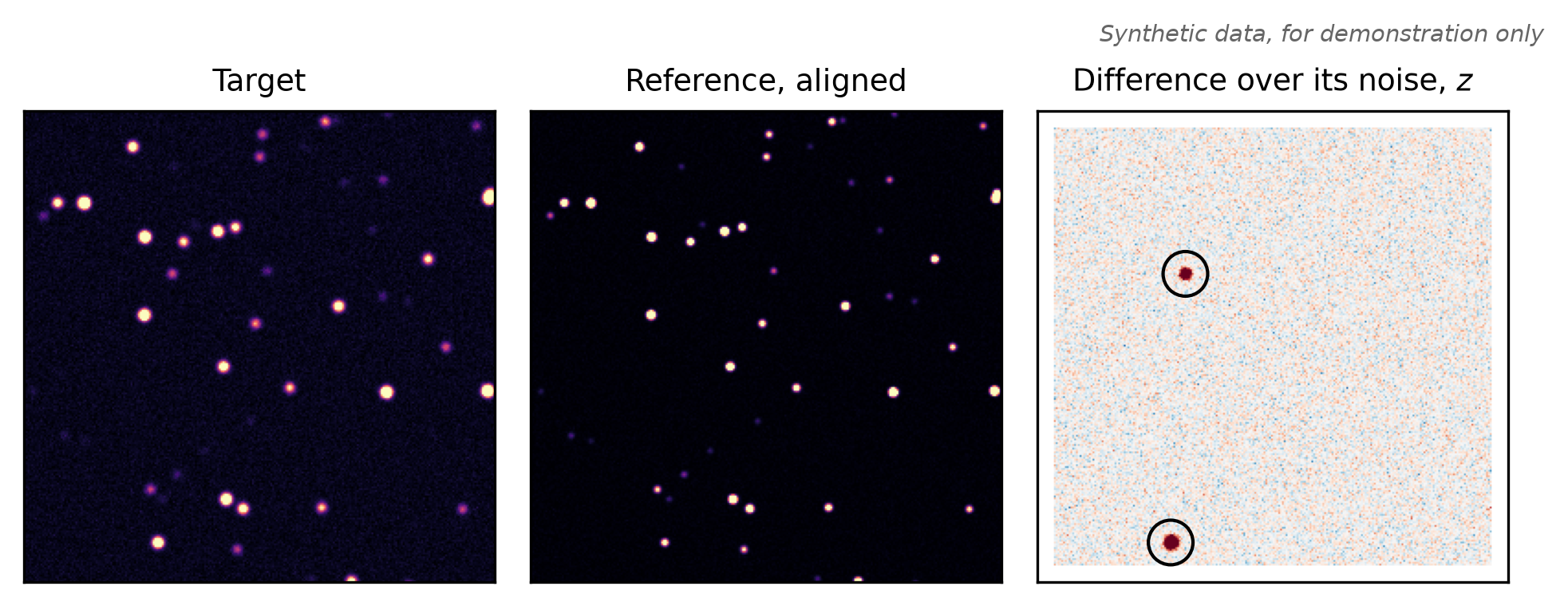
Two regions pass the threshold of 5 in this sample: the brightened star and the new source. This threshold is in the approximate noise units of z; it does not by itself set a false-detection probability.
2.7 Measure the candidates
xFit fits a model to a batch of cutouts at once. window_stamps from xPois cuts a square window around each position, with NaN where the window leaves the image. Cut the difference and its predicted variance the same way, then fit one Gaussian source per cutout. The fit returns each source’s flux and its error.
sources.flux is a nonnegative magnitude; the fitted amplitude supplies the sign above. These are difference fluxes: the change in flux between the target and the matched reference. Check sources.converged and sources.uncertainty_valid before using their errors. Those formal errors use the supplied diagonal variance and fixed Gaussian PSF; Chapter 10 describes additional terms. The third argument is each source’s starting position, as (x, y) pixels from the cutout center. psf_sigma fixes the width of the source to the target’s PSF (point spread function: the blur pattern of a point of light).
2.8 Look at the result
Figure 2.1 shows the inputs and the difference image.
Plotting code
import matplotlib.pyplot as pltfig, axes = plt.subplots(1, 3, figsize=(6.5, 2.5))lo, hi = np.percentile(target, [1, 99.5])for ax, image, title in [(axes[0], target, "Target"), (axes[1], aligned.image, "Reference, aligned")]: ax.imshow(image, origin="lower", cmap="magma", vmin=lo, vmax=hi) ax.set_title(title, fontsize=9)axes[2].imshow(z, origin="lower", cmap="RdBu_r", vmin=-6, vmax=6)axes[2].scatter(peaks[:, 1], peaks[:, 0], s=180, facecolors="none", edgecolors="black", linewidths=1)axes[2].set_title("Difference over its noise, $z$", fontsize=9)for ax in axes: ax.set_xticks([]); ax.set_yticks([])fig.text(1, 1, "Synthetic data, for demonstration only", ha="right", va="bottom", fontsize=7, style="italic", color="0.4", transform=fig.transFigure)fig.tight_layout()plt.show()
Figure 2.1: The sample pair at three stages. Left: the target. Middle: the reference after xRep, on the target grid. Right: the standardized difference \(z\) on a red-blue scale from -6 to 6, with the two candidates circled. The two injected changes stand out against the residual background. The white frame is the edge band the kernel cannot reach. Synthetic data, for demonstration only.
2.9 Run it on a GPU
On a host with the gpu profile, select the GPU backends. xRep and xPois take a backend argument. xRep returns host (NumPy) arrays. xFit runs on the device when you pass it CuPy arrays, and returns CuPy arrays.