xImage makes one sharp image from many registered frames with known PSFs (point spread functions: the blur pattern of a point of light in each frame). It fits one nonnegative scene that, blurred by each frame’s PSF, matches every frame within its noise. Use it when you have several exposures of the same field on one pixel grid, each with its own blur and noise. xImage runs on PyTorch, on a CPU or a CUDA GPU. Each workflow reads a bundle of arrays and a YAML configuration, then writes a run directory with a receipt.
You need:
cuPhoton with the ximage extra, which adds PyTorch, Photutils and Zarr (Chapter 1).
Frames already on one pixel grid (Chapter 5), a variance plane per frame and one PSF per frame.
The cuPhoton checkout, for its example configurations. Run from the root of your checkout, or set CUPHOTON_REPO to its path.
NoteSample data
This page runs on a small synthetic bundle. The printed values only demonstrate the API.
11.1 Make the frames
The block below makes three noisy 64 by 64 frames of three point sources. Each frame has its own Gaussian PSF, 0.8, 1.0 and 1.2 pixels wide. These are the same arrays that the repository’s examples/ximage/make_synthetic_bundle.py writes.
A bundle is a set of named arrays in one NPY directory, HDF5 file or Zarr store. Three arrays are required:
Key
Axes
Holds
images
(batch, y, x, frame)
the registered frames
variances
(batch, y, x, frame)
the variance of every pixel, finite and positive
psfs
(psf_y, psf_x, channel, frame)
one PSF per frame, square, odd-sized, one channel
An NPY bundle is a directory with one <key>.npy file per array. validate_bundle checks the array layout, mask dtype and exposure times and returns a list of issues. An empty list does not check every pixel value; check that the image and variance values are usable before reconstruction. summarize_bundle returns each array’s shape, dtype and axes.
from pathlib import Pathfrom cuphoton.ximage import load_ximage_bundle, summarize_bundle, validate_bundlebundle_dir = Path("sample/ximage")bundle_dir.mkdir(parents=True, exist_ok=True)np.save(bundle_dir /"images.npy", images)np.save(bundle_dir /"variances.npy", np.full_like(images, 0.01**2))np.save(bundle_dir /"psfs.npy", psfs)with load_ximage_bundle(bundle_dir) as bundle:print("issues:", validate_bundle(bundle))for key, info in summarize_bundle(bundle).items():print(f"{key:9s}{info['shape']}{info['axes']}")
Optional arrays use the same naming. masks is a boolean array shaped like images, True for a good pixel. exp_times holds one positive value per frame. xImage divides each frame by its exposure time and each variance by its square. The data contract lists every array.
11.3 Write a configuration
A workflow reads its settings from a YAML file. xImage validates the file strictly. A misspelled key is an error. The repository has annotated examples in examples/ximage/. Copy the L2 example, point it at the bundle, and give the run a name that later runs can overwrite:
The example reconstructs the central 48 by 48 pixels. With VALID padding, the frames must hold real pixels half a PSF beyond each edge of the region, 4 pixels for these 9 by 9 PSFs. device: auto runs on CUDA when PyTorch sees a GPU and on the CPU otherwise. Table 11.1 lists the keys you change first.
11.4 Run the reconstruction
run_reconstruction takes the configuration’s path as a Path. It returns a WorkflowResult with the run directory and the summary, which the run also saves as its receipt.
from cuphoton.ximage.workflows import run_reconstructionresult = run_reconstruction(Path("sample/reconstruct-l2.yaml"))summary = result.summaryprint(result.run_dir.name, summary["backend"], summary["performance"]["device"]["device"], summary["dtype"])print("saved image:", summary["image_shape"])trace = summary["trace_summary"]print(f"{trace['iterations_count']} iterations, loss {trace['loss_last']:.2f}, u_score {trace['u_score_last']:.1e}")
l2 torch cpu float64
saved image: [1, 56, 56, 1]
75 iterations, loss 2.97, u_score 7.9e-06
The saved image is the 48-pixel region plus the 4-pixel PSF border on each side. A run stops after max_iter iterations, or earlier once the update score u_score falls below stop_tol. The loss is the mean, over good pixels, of the squared residual divided by the variance.
11.5 Read the run directory
This reconstruction writes the following files:
print(sorted(str(p.relative_to(result.run_dir)) for p in result.run_dir.rglob("*") if p.is_file()))image = np.load(summary["saved"]["image"])scene_l2 = image[0, 4:-4, 4:-4, 0] # drop the 4-pixel PSF borderprint(image.shape, "->", scene_l2.shape)
config.yaml: the configuration as the run resolved it, with every default filled in.
summary.json: the receipt. It records the backend, device, dtype, cuPhoton version, input store, region, saved paths, a trace summary and timings.
artifacts/image.npy: the scene on the region plus its border.
trace/: the loss and update score at each iteration.
Crop the border before you use the scene, as the evaluation does. The scene is in exposure-time-normalized units. The run returns no output variance and no effective PSF for the scene. summary.json holds input paths and metadata. Review it before you share it.
11.6 Evaluate the run
evaluate_reconstruction_run crops the scene to the region and compares it with a median coadd (the pixel-by-pixel median of the frames). It reports sharpness, sky scatter, PSNR and SSIM (two image-similarity scores), and the flux of detected sources.
from cuphoton.ximage.evaluation import evaluate_reconstruction_runevaluation = evaluate_reconstruction_run(result.run_dir, metrics_backend="auto")print(evaluation["metrics_backend"], evaluation["projection_shape"])for name in ("restoration", "synthetic_coadd"):print(name, {key: round(value, 3) for key, value in evaluation[name].items() ifisinstance(value, float)})print("matched sources:", evaluation["photometry"]["matched_aperture_count"])
restoration describes the scene and synthetic_coadd the median. Both come from the same frames and share their noise. Similarity or sharpness alone therefore does not show that a reconstruction is accurate.
11.7 Calibrate the PSFs
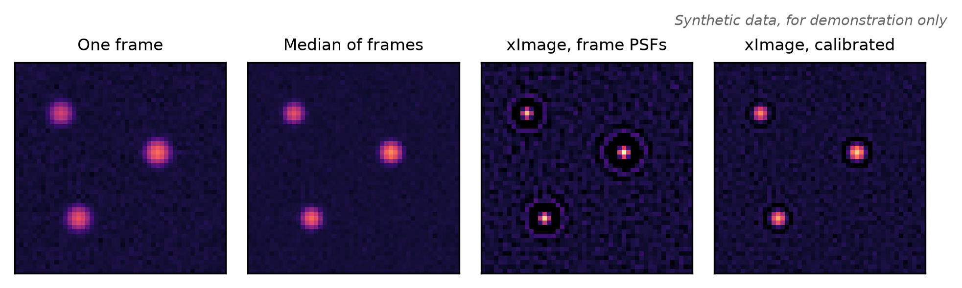
With the frame PSFs, xImage aims for the scene itself, with point sources as single pixels. PSF calibration instead fits, for each frame, the kernel that blurs a narrow Gaussian of width sigma_g (0.55 pixels in the example) into that frame’s PSF. A reconstruction with these kernels returns the scene as seen through that Gaussian. run_psf_solve fits them with multiplicative updates (method: mm) or the Adam optimizer (method: adam).
from cuphoton.ximage.workflows import run_psf_solvepsf_config = yaml.safe_load((REPO /"examples/ximage/psf-mm.example.yaml").read_text())psf_config["data"]["base"] ="sample/ximage"psf_config["output"] = {"root_dir": "sample/runs", "name": "psf-mm", "overwrite": True}Path("sample/psf-mm.yaml").write_text(yaml.safe_dump(psf_config, sort_keys=False))kernels = run_psf_solve(Path("sample/psf-mm.yaml"))print(kernels.summary["method"], kernels.summary["psfs_shape"])print(sorted(p.name for p in (kernels.run_dir /"artifacts").iterdir()))
mm [9, 9, 1, 3]
['gaussian_psf.npy', 'psfs.npy', 'psfs_padded.npy']
psfs.npy holds the kernels, psfs_padded.npy the kernels before their final crop, and gaussian_psf.npy the Gaussian. To reconstruct with the kernels, set psf_path to the saved psfs.npy:
Figure 11.1: The central 48 by 48 pixels of the sample bundle on one logarithmic color scale, brighter for higher intensity. From left: the frame with the widest PSF, the median of the three frames, the L2 reconstruction with the frame PSFs, and the L2 reconstruction with calibrated kernels. With the frame PSFs, each source shrinks to a few pixels inside a dark ring where the scene falls below the sky level. The calibrated reconstruction shows each source as a slightly wider spot. Synthetic data, for demonstration only.
11.9 Options
Table 11.1: Reconstruction keys to change first. The examples set roi to 48 by 48 and mask.mode to none.
Key
Default
Effect
algorithm
set by the command
l2 (variance-weighted least squares) or rho (robust loss)
device
auto
cpu, cuda, or auto (CUDA when PyTorch sees a GPU)
dtype
float64
float32 or float64
data.base
data
the bundle path, relative to the working directory
data.exposure_indices, data.max_exposures
null
use a subset of the frames (set one, not both)
output.root_dir
~/.local/state/cuphoton/ximage/runs
where runs go (under $XDG_STATE_HOME when set)
output.name, output.overwrite
null, false
the run directory name (timestamped when null), and whether to replace it
roi.center, roi.height, roi.width
null
the region in pixels, center as (row, column). null means the whole frame and its middle
mask.mode
provided
provided uses the bundle’s masks, none ignores them
psf_path
null
calibrated kernels from a PSF run, or null for the bundle’s PSFs
max_iter, stop_tol
75, 1e-6
the iteration cap, and the update score below which a run stops early
padding
VALID
VALID needs real pixels half a PSF beyond the region, SAME treats them as zero
exposure_batch_size
null
frames per convolution call, null for all at once
rho_loss
huber
the loss for rho runs. cauchy, bisquare and damped_rl are experimental
delta_rho_start, delta_rho_end
2.0, 1.0
the Huber threshold in standard deviations, lowered linearly over the iterations
rho applies the Huber loss to each residual divided by its noise. The loss is quadratic up to the threshold and linear beyond it. A few large residuals therefore pull less on the scene. reconstruct-rho.example.yaml sets it up. For the PSF calibration keys, refer to the annotated psf-mm.example.yaml and psf-adam.example.yaml.
11.10 On a GPU
Use the GPU environment from Chapter 1, which includes ximage and the plotting dependencies.
device_override="cuda" (or device: cuda) requires a GPU. metrics_backend="cupy" computes the evaluation metrics on it:
To reduce convolution working memory, set exposure_batch_size to a positive number of frames. The selected input images, variances and masks still reside on the device together. Use a smaller region, fewer frames or tiling to reduce that input footprint. The receipt records the resolved device, precision and timings. The evaluation records metrics_backend separately from the reconstruction backend.
11.11 Command line
The cuphoton ximage commands run the same workflows. From the root of the checkout, the repository’s example runs end to end:
uv run --no-sync python examples/ximage/make_synthetic_bundle.py --output datauv run --no-sync cuphoton ximage data-validate --base datauv run --no-sync cuphoton ximage reconstruct-l2 --config examples/ximage/reconstruct-l2.example.yamluv run --no-sync cuphoton ximage psf-solve-mm --config examples/ximage/psf-mm.example.yamluv run --no-sync cuphoton ximage evaluate-reconstruction --run-dir runs/reconstruct-l2-example
data-validate prints each array’s shape or the list of issues. The reconstruction and PSF commands print the run summary and accept --device, --backend and --output-dir overrides. evaluate-reconstruction also writes evaluation/evaluation_summary.json into the run directory. The example script and configurations do not overwrite earlier output. To repeat them, use a new bundle path and run names, or remove only the outputs created by this example. To time a workflow on the CPU and the GPU, run benchmark-devices:
The xImage reference covers HDF5 and Zarr bundles, tiling, the survey adapters and the evaluation’s catalog comparisons.
xImage adapts the ImageMM method of Sukurdeep et al. (2025). If you publish results, cite ImageMM and your cuPhoton version, as the citation guide describes.