xray doctor

Runtime:
  Python: 3.12.3
  cuPhoton: 0.3.0.dev98+gc04d1a5
  NumPy: 2.4.6
  CuPy: not installed

Capabilities:
  ok      numpy          [required] array operations
  ok      h5py           [required] HDF5 input
  missing cupy           [gpu] CUDA array kernels
  missing bokeh          [optional] interactive review views

Executables:
  missing nvidia-smi
  missing sbatch

CUDA visibility: empty12 Analyze X-ray detector traces
xRay (cuphoton.xray) analyzes time-resolved X-ray detector data from pump-probe scans. A laser pulse excites the sample (the pump), and an X-ray pulse a set delay later records it on an area detector (the probe). Each delay gives one detector frame. You reduce a laser-on and laser-off pair of frame stacks to a trace and fit it as a sum of damped oscillations. On a GPU, the same fit runs on every detector row.
You need:
- cuPhoton with the CPU profile (Chapter 1) for the trace steps.
- The
gpuprofile and an NVIDIA GPU for the default detector-wide fit. The restrictedstructured-cpubackend is a separate option (Section 12.9). - A laser-on and laser-off pair of HDF5 files (Hierarchical Data Format 5, a format for named arrays), or the sample pair below.
NoteSample data
This page runs on a small synthetic pair. The printed values only demonstrate the API.
12.1 Check the environment
Run the xRay doctor on a new machine. It lists the libraries xRay found:
cuphoton xray doctorNumPy and h5py are required. The trace steps below run without CuPy; the GPU trace API and default detector-wide backend require it. Bokeh adds interactive review pages. Include this output in environment bug reports.
12.2 Make a sample pair
xRay reads two layouts of laser-on and laser-off files. Both files in a pair must use the same layout, the same frame shape and the same delays. The sample pair uses the cropped-cube layout:
| Dataset | Shape | Holds |
|---|---|---|
imgs |
(frame, y, x) | the detector image at each delay |
scan_var |
(frame,) | the pump-probe delay, in the file’s own units |
i0 |
(frame,) | the incident-beam monitor. xRay divides each frame’s sum by it. |
i0_ipm3 |
(frame,) | a second monitor, required by the layout check |
bin_count |
(frame,) | entries per frame, required by the layout check |
ROI |
any | the region stored with the cube, required by the layout check |
The xRay guide describes the other layout, legate-cube. The block below writes xray-sample/on.h5 and xray-sample/off.h5. The laser-on frames change by two damped oscillations and a small constant, on top of Poisson counts.
Create the sample pair (NumPy and h5py only)
# Writes xray-sample/on.h5 and xray-sample/off.h5: 97 delay frames of a 32 x 32
# detector. The laser-on frames change by two damped oscillations and a constant.
from pathlib import Path

import h5py
import numpy as np

rng = np.random.default_rng(5)
frames, height, width = 97, 32, 32
delay = (np.arange(frames) - 1) * 0.1  # ps; xRay drops frame 0 by default
t = np.clip(delay, 0.0, None)
change = (0.04 * np.exp(-0.15 * t) * np.cos(2.0 * t + 0.3)
          + 0.02 * np.exp(-0.08 * t) * np.cos(4.5 * t - 0.75) + 0.01)

Path("xray-sample").mkdir(exist_ok=True)
for name, factor in (("on", 1.0 + change), ("off", np.ones(frames))):
    i0 = 1.0e4 * (1.0 + 0.03 * rng.standard_normal(frames))  # incident-beam monitor
    counts = 5.0e4 * (i0 / 1.0e4 * factor)[:, None, None] * np.ones((height, width))
    with h5py.File(f"xray-sample/{name}.h5", "w") as h5:
        h5["imgs"] = rng.poisson(counts).astype(np.float32)
        h5["scan_var"] = delay
        h5["i0"] = i0
        h5["i0_ipm3"] = i0
        h5["bin_count"] = np.full(frames, 50)
        h5["ROI"] = np.array([0, 0, width, height])
Probe the pair before an analysis. probe_hdf5_pair reports the layout of each file and the monitor xRay normalizes by:
from cuphoton.xray.hdf5 import probe_hdf5_pair

probe = probe_hdf5_pair(h5dir="xray-sample", fon="on.h5", foff="off.h5")
for side in (probe.on, probe.off):
    print(side.path.name, side.schema, "normalized by", side.load_plan.ipm_pair.normalization)
on.h5 cropped-cube normalized by i0
off.h5 cropped-cube normalized by i0A file that xRay does not recognize reports unknown.
12.3 Extract a trace
load_hdf5_pair_roi_trace reduces the pair to one trace for a region of interest (ROI). Give the ROI’s origin (roi_x, roi_y) and size (roi_width, roi_height) in detector pixels. The block takes one 16 × 16 pixel tile:
from cuphoton.xray.hdf5 import load_hdf5_pair_roi_trace

pair = load_hdf5_pair_roi_trace(h5dir="xray-sample", fon="on.h5", foff="off.h5",
                                roi_x=0, roi_y=0, roi_width=16, roi_height=16)
delay, trace = pair.delay, pair.ratio_minus_one
print(f"{delay.size} samples, delay {delay[0]:.1f} to {delay[-1]:.1f} ps")
print(f"trace from {trace.min():.4f} to {trace.max():.4f}")
96 samples, delay 0.0 to 9.5 ps
trace from -0.0142 to 0.0319xRay drops the first frame, sums the ROI’s pixels in each frame and divides each sum by i0. It then forms (on + S) / (off + S) - 1, where S is the mean laser-off sum. With this reference shift, the trace is about half the relative change of the laser-on frames. Pass reference_shift=False for on / off - 1. Delays keep the file’s units, picoseconds here. load_hdf5_pair_trace reduces the whole detector instead.
12.4 Choose the model order
Linear prediction fits a sum of damped cosines plus a constant with no starting guess. It assumes finite samples at uniformly increasing delays; check that condition before fitting your own trace. It turns the fit into linear algebra and reads each mode’s frequency and decay rate from the roots of a polynomial. The one choice you make is the model order, n_components, the number of singular values the fit keeps. Each oscillating mode adds two to the order. Too small an order misses a mode, and too large an order fits noise.
model_order_sweep fits the trace at each requested order. It picks the smallest order whose RMS (root-mean-square) residual is within 1% of the best:
from cuphoton.xray.linear_prediction import model_order_sweep

sweep = model_order_sweep(delay, trace, tuple(range(1, 10)))
for entry in sweep.entries:
    print(f"order {entry.components}: RMS residual {entry.rms_residual:.2e}")
print("chosen order:", sweep.best_components)
order 1: RMS residual 1.00e-02
order 2: RMS residual 1.00e-02
order 3: RMS residual 1.75e-03
order 4: RMS residual 1.91e-04
order 5: RMS residual 1.91e-04
order 6: RMS residual 1.91e-04
order 7: RMS residual 1.91e-04
order 8: RMS residual 1.91e-04
order 9: RMS residual 1.91e-04
chosen order: 4The chosen order balances residual size against model order among the values tested. Set relative_tolerance to change the 1% rule.
12.5 Fit the trace with linear prediction
Fit the trace at the chosen order and print each mode:
from cuphoton.xray.linear_prediction import linear_prediction_numpy

fit = linear_prediction_numpy(delay, trace, sweep.best_components)
for w, g, a in zip(fit.angular_frequency, fit.decay, fit.amplitude):
    print(f"{w / (2 * np.pi):.3f} THz, decay {g:.3f} per ps, amplitude {a:.4f}")
0.318 THz, decay 0.148 per ps, amplitude 0.0199
0.717 THz, decay 0.079 per ps, amplitude 0.0099The fit returns these fields, all as NumPy arrays or numbers:
| Field | Holds |
|---|---|
angular_frequency |
each mode’s angular frequency, in radians per delay unit |
decay |
each mode’s decay rate, in inverse delay units |
amplitude, phase |
each mode’s amplitude (trace units) and phase (radians, at the first sample) |
reconstruction |
the fitted modes plus the constant, on fit.time |
frequency, spectrum_total |
the modal spectrum, on a grid in cycles per delay unit |
chi2 |
sum of squared residuals over the first N − 1 samples, divided by N − 2, where N is the trace length; no variance weighting |
selected_model_order |
the order used |
Divide angular_frequency by 2π for cycles per delay unit. With delays in picoseconds, that is THz. fit.time starts at zero on the first sample. Section 12.9 lists the call’s options.
12.6 Look at the fit
Figure 12.1 shows the trace, the fit and the spectrum of the fitted modes.
Plotting code
import matplotlib.pyplot as plt

fig, (ax_t, ax_f) = plt.subplots(1, 2, figsize=(6.5, 2.6))
ax_t.plot(delay, trace, ".", color="0.5", ms=3, label="trace")
ax_t.plot(fit.time + delay[0], fit.reconstruction, color="#2A78D6", lw=1.2, label="fit")
ax_t.set_xlabel("Delay (ps)")
ax_t.set_ylabel("Trace")
ax_t.legend(frameon=False, fontsize=8)
ax_f.plot(fit.frequency, fit.spectrum_total, color="#2A78D6", lw=1.2)
ax_f.set_xlabel("Frequency (THz)")
ax_f.set_ylabel("Modal spectrum")
fig.text(1, 1, "Synthetic data, for demonstration only", ha="right", va="bottom",
         fontsize=7, style="italic", color="0.4", transform=fig.transFigure)
fig.tight_layout()
plt.show()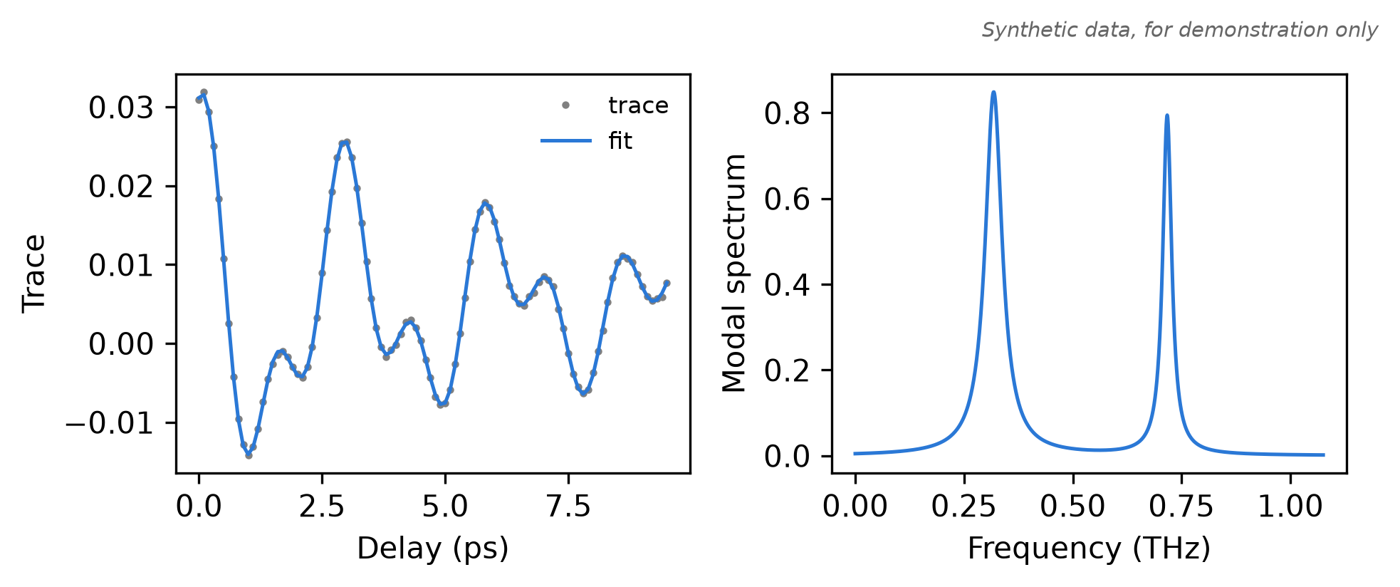
The reconstruction should follow the points with no leftover oscillation. For a missing mode, refer to Section 12.12.
12.7 Fit every detector row
detector-artifacts runs the fit across a region of the detector, in tiles of 16 × 16 pixels by default. For each detector row of each tile, it does the following:
- Sums the tile’s columns and the rows within
--integratepixels (3 by default). - Smooths the trace along the delay with a Savitzky-Golay filter (a sliding polynomial fit).
- Fits the trace, starting at the
--zero-offset-indexsample. - Writes the result to every column of the tile.
These steps change the trace’s support and amplitude. Detector fits therefore differ from a fit of the tile trace above. Plan the run first. detector-mask counts the tiles and row fits on the CPU:
cuphoton xray detector-mask --roi-lower 0 0 --roi-dim 32 32roi=[0:32,0:32]
tile_size=16x16
exclude_y=
total_tiles=4
active_tiles=4
fully_excluded_tiles=0
partially_excluded_tiles=0
total_row_fits=64
active_row_fits=64
skipped_row_fits=0Add --exclude-y start:end to skip dead detector rows. This fit uses the default backend, which needs CuPy and a GPU:
cuphoton xray detector-artifacts --h5dir xray-sample --fon on.h5 --foff off.h5 \
  --output-dir xray-artifacts --roi-lower 0 0 --roi-dim 32 32 \
  --zero-offset-index 0 --components 4 --fit-diagnostics summary --artifact-layout tile-rows
--zero-offset-index is the first fitted sample, counted after the dropped frame. Choose a fit start that suits your scan. The fit also drops the last sample (--fit-trailing-drop 1) and needs at least 16 samples. Set --components to the order the sweep chose. The default is 30. Check the outputs of a small ROI before you run the whole detector.
12.8 Read the outputs
detector-artifacts writes these files to --output-dir:
| File | Shape | Holds |
|---|---|---|
manifest.json |
the inputs, ROI, fit settings, counts of fits and failures, and the status codes | |
freq_all.npy |
(y, x, mode) | each mode’s peak frequency on the sampled modal spectrum, in cycles per delay unit, zero-padded; iterative fits store the fitted frequency directly |
amp_all.npy |
(y, x, mode) | each fitted mode’s amplitude, zero-padded |
fft_all.npy, fft_freq_all.npy |
(y, x, bin) | the magnitude of the trace’s Fourier transform, and its frequencies |
amp_all_sum_filtered.npy |
(y, x) | the sum of amplitudes strictly above --amp-threshold (default 1.6) and below 1e6 |
fit_status.npy |
(y, x) | 0 not processed, 1 fitted, 2 skipped, 3 failed |
fit_diagnostics.npz |
per-row residual and conditioning records, with --fit-diagnostics summary or full |
|
spectral-layout.json |
the tile map, with --artifact-layout tile-rows |
The default dense layout stores each spectrum at every pixel. tile-rows stores it once per tile row, in *.tile-rows.npy files. load_detector_array reads either layout by its plain name and expands only the slice you index:
from cuphoton.xray.detector_storage import load_detector_array

freq = load_detector_array("xray-artifacts/freq_all.npy")  # opens freq_all.tile-rows.npy
column = freq[:, 8, :3]  # NumPy array: the first three modes of column 8, every row
status = np.load("xray-artifacts/fit_status.npy")
print(column.shape, np.unique(status))
Converting the whole compact array, as in np.asarray(freq), raises TypeError. Index a slice first. Indices are local to the ROI. Add the manifest’s roi_lower, an (x, y) origin, for detector pixels. For an interactive view of one column, install the viz extra and run:
cuphoton xray phonon-viz --detector-artifact-dir xray-artifacts --x-value 8 --output phonon.html12.9 Options
load_hdf5_pair_roi_trace takes these options besides the files and the ROI:
| Option | Default | Effect |
|---|---|---|
row_y |
None |
One absolute detector row inside the ROI, instead of the whole ROI |
exclude_y |
() |
Detector row ranges to leave out of the sums |
drop_leading |
1 |
Leading frames to drop |
reference_shift |
True |
Add the mean laser-off level to both sides of the ratio |
linear_prediction_numpy and linear_prediction_cupy take these options:
| Option | Default | Effect |
|---|---|---|
n_components |
required | Model order: the number of singular values kept. Each oscillating mode adds two. |
roots_backend |
"eigvals" |
Root solver. "eigvals" takes companion-matrix eigenvalues. "roots" uses NumPy or CuPy roots, matching the array backend. |
p2_ridge_alpha |
0.0 |
Ridge penalty on the fitted cosine and sine terms. The constant is never penalized. |
fit_diagnostics |
False |
Fill fit.diagnostics with residual and conditioning metrics |
detector-artifacts takes these fit options:
| Option | Default | Effect |
|---|---|---|
--tile-shape |
16 16 |
Tile width and height. One fit per detector row of each tile. |
--integrate |
3 |
Row radius summed into each row’s trace |
--savgol-window, --savgol-polyorder |
5, 3 |
Savitzky-Golay smoothing before the fit |
--components |
30 |
Model order, or the mode count for the iterative fit |
--fit-method |
linear-prediction |
iterative fits a fixed number of modes by Levenberg-Marquardt iteration |
--fit-backend |
cupy |
structured-cpu and structured-gpu need the native extension, a 798-sample fitted window, tiles of at most 16 by 16, batched rows, and the default --fit-method, --components, --fit-diagnostics, --p2-ridge-alpha and --roots-backend. Distributed runs reject them. |
--structured-schedule |
serial |
overlap overlaps one GPU root batch with host work, on structured-gpu only |
--artifact-layout |
dense |
tile-rows stores each spectrum once per tile row |
--fit-diagnostics |
none |
summary or full records per-row diagnostics |
--max-fit-failures |
0 |
Failed row fits allowed before the command fails |
Set CUPHOTON_XRAY_HDF5_SELF_CONTAINED=1 to reject inputs that link to other files. By default, xRay follows HDF5 links, external storage and virtual datasets.
12.10 On a GPU
With the gpu profile, linear_prediction_cupy runs the same fit on CuPy and returns NumPy arrays. build_detector_artifacts_cupy is the Python form of detector-artifacts:
from cuphoton.xray.detector_artifacts import build_detector_artifacts_cupy
from cuphoton.xray.linear_prediction import linear_prediction_cupy

fit = linear_prediction_cupy(delay, trace, 4)
result = build_detector_artifacts_cupy(
    h5dir="xray-sample", fon="on.h5", foff="off.h5", output_dir="xray-artifacts",
    roi_lower=(0, 0), roi_dim=(32, 32), zero_offset_index=0, components=4,
    fit_diagnostics="summary", artifact_layout="tile-rows",
)
print(result.manifest_path, result.raw_fits, result.failures)
To split a large detector across GPUs or Slurm jobs, use detector-artifact-distributed (Chapter 14).
12.11 Command line
extract-trace writes a trace to an NPZ file with time, trace and summary entries. model-order-sweep reads it:
cuphoton xray extract-trace --h5dir xray-sample --fon on.h5 --foff off.h5 \
  --roi-lower 0 0 --roi-dim 16 16 --output tile.npz
cuphoton xray model-order-sweep --trace-npz tile.npz --min-components 2 --max-components 8 --step 2
artifact=tile.npz
samples=96
source=hdf5-roi
roi_lower=[0, 0]
roi_dim=[16, 16]
row_y=None
delay_range=0.0:9.5
ratio_range=-0.014159337794647064:0.0051055214589572386:0.03190378806283012
source=trace-npz
samples=96
roots_backend=eigvals
best_components=4
best_selected_model_order=4
best_rms_residual=0.00019135
best_reconstruction_rms_error=0.00019135
components=2 selected_model_order=2 rms_residual=0.0100493 reconstruction_rms_error=0.0100493 chi2=0.000103065 selected_roots=0 decaying_roots=0
components=4 selected_model_order=4 rms_residual=0.00019135 reconstruction_rms_error=0.00019135 chi2=3.73938e-08 selected_roots=2 decaying_roots=4
components=6 selected_model_order=6 rms_residual=0.000190663 reconstruction_rms_error=0.000190663 chi2=3.70897e-08 selected_roots=2 decaying_roots=4
components=8 selected_model_order=8 rms_residual=0.000190992 reconstruction_rms_error=0.000190992 chi2=3.72241e-08 selected_roots=3 decaying_roots=5data-probe prints the same check as probe_hdf5_pair. To write one trace per detector row, repeat --row-y with --output-dir, keeping --roi-lower and --roi-dim to define the containing ROI. model-order-sweep --trace-dir sweeps that directory. Add --json for machine-readable output. cuphoton xray --help lists every command.
12.12 Troubleshooting
CuPy is required for detector artifacts. Install thegpuprofile, or fit single traces on the CPU withlinear_prediction_numpy.The structured xRay backend requires the native extension. SetCUPHOTON_XRAY_BUILD_EXT=1and add--reinstall-package cuphotonto youruv synccommand, retaining the extras you need. The build needs Linux and a C++17 compiler.time and trace must contain at least 16 samples. Use a longer scan.on/off delay axes do not match, orschema mismatch. The files come from different scans or layouts. Rundata-probe.- A fast mode is missing from the fit. Linear prediction keeps only part of the polynomial’s roots, prioritizing large real parts, then filters by decay. This can discard high-frequency modes even without noise; there is no fixed frequency cutoff that guarantees recovery. Check synthetic modes at your scan’s sampling cadence, or try
--fit-method iterative. Its frequency bound is the Nyquist frequency (half the sampling rate) by default. Bokeh is required for phonon-viz. Install thevizextra.
12.13 Next steps
- Run detector fits on many GPUs or Slurm nodes: Chapter 14 and the distributed detector guide.
- Check linear prediction against synthetic modes with
cuphoton xray lpv: the validation guide. - The full reference, with the iterative fit and the structured backends: the xRay guide.
- Correlate two sampled signals instead of fitting one: Chapter 13.