DISCO convolutions on the sphere

This guide explains the discrete-continuous (DISCO) convolution implemented in DiscreteContinuousConvS2. We start with the mathematical formulation, show how the filter basis functions look, and walk through a concrete convolution example.

1. Convolution on the sphere

A convolution on \(S^2\) generalises the familiar planar convolution by replacing translations with rotations. Given a multi-channel input signal \(f^{c_i}(\omega)\) and a filter \(\kappa\) centred at the north pole, the output at point \(\omega'\) is

\[ g^{c_o}(\omega') = \sum_{c_i} \int_{S^2} \kappa^{c_o,c_i}\!\bigl(R_{\omega'}^{-1}\,\omega\bigr)\; f^{c_i}(\omega)\;\mathrm{d}\omega \]

where \(\omega = (\theta, \lambda)\) are coordinates on the sphere and \(R_{\omega'}\) is the rotation that maps the north pole to the output point \(\omega'\). Evaluating this integral naively for all output points would be \(O(N^2)\) in the number of grid points.

Making it tractable

The DISCO approach (Ocampo, Price & McEwen, ICLR 2023) makes two key choices:

1. Compact support – the filter \(\kappa\) is non-zero only within an angular cap of radius theta_cutoff around the north pole. This means each output point only “sees” a small, fixed-size neighbourhood of input points, reducing the cost to \(O(N)\).

2. Continuous parameterisation – the filter is expressed as a learnable linear combination of fixed basis functions \(\{\phi_k\}\):

\[ \kappa^{c_o, c_i}(\vartheta, \varphi) = \sum_{k=0}^{K-1} w_k^{c_o, c_i}\;\phi_k(\vartheta, \varphi) \]

where \(\vartheta\) is the angular distance from the filter centre and \(\varphi\) the azimuthal angle. Because the filter is defined continuously (not on a fixed grid), the same weights \(w_k\) can be evaluated on different input/output resolutions.

2. The \(\Psi\) convolution tensor

To evaluate the integral numerically, the basis functions \(\phi_k\) are sampled at the rotated positions of the input grid points. For each output latitude \(\theta'_j\), the rotation \(R_{\omega'_j}^{-1}\) maps each input point \((\theta_i, \lambda_p)\) into the filter’s local frame. The basis function values at those positions, multiplied by the quadrature weights \(q_i\), form the sparse convolution tensor:

\[ \Psi_{k,\,j,\,(i,p)} = \phi_k\!\bigl(\vartheta(\theta'_j, \theta_i, \lambda_p),\; \varphi(\theta'_j, \theta_i, \lambda_p)\bigr) \; q_i \]

Two important properties make this efficient:

• Sparsity: because of the compact support, most entries of \(\Psi\) are zero. Only the input points that fall inside the angular cap contribute.

• Longitude invariance (p-shift): because the grid is equispaced in longitude, \(\Psi\) does not depend on the output longitude \(\lambda'\). Shifting \(\lambda'\) simply shifts which input longitudes contribute. This reduces storage by a factor of \(N_{\lambda,\text{out}}\).

Forward pass

The full forward pass is then a sparse contraction (over the input grid) followed by a dense channel-mixing matrix multiply:

\[ g^{c_o}(\theta'_j, \lambda'_q) = \sum_{c_i} \sum_k w_k^{c_o,c_i} \sum_{i,p} \Psi_{k,j,(i,p)}\; f^{c_i}(\theta_i, \lambda'_q + \lambda_p) \]

Because \(\Psi\) is sparse (compact support) and independent of \(\lambda'\) (p-shift), cost and memory scale linearly in the number of grid points.

Equivariance

Keeping the filter continuous makes the convolution approximately \(SO(3)\)-equivariant (rotations of the filter are restricted to the quotient \(SO(3)/SO(2)\)), while the discrete quadrature makes it scalable to high resolution – reconciling the equivariance-versus-scalability trade-off of earlier spherical CNNs. Since the filter is continuous, the layer is also resolution-agnostic: the same learned weights can be evaluated on different input/output grids (grid_in/grid_out), though the learned features themselves remain resolution dependent.

3. Filter basis functions

The choice of basis functions \(\phi_k\) is controlled by the basis_type parameter (see get_filter_basis()). All bases are defined on a disk of unit radius (mapped to the spherical cap \([0, \theta_\text{cutoff}]\)) and have compact support. torch-harmonics provides four built-in bases:

basis_type	Description	kernel_shape
"piecewise linear"	Tensor-product hat functions on a polar grid	(n_radial, n_angular)
"harmonic"	Hann-windowed Fourier modes (L2-normalised)	(n_radial, n_angular)
"zernike"	Zernike polynomials on the unit disk	n_max (scalar)
"fourier-bessel"	Fourier–Bessel functions \(J_m(\alpha_{m,n}\,r)\cos(m\varphi)\)	(n_radial, n_angular)

Let’s visualise each of them.

import math

import matplotlib.pyplot as plt
import numpy as np
import torch

from torch_harmonics.filter_basis import get_filter_basis
from torch_harmonics.plotting import plot_sphere

cmap = plt.cm.RdBu

def evaluate_basis(fb, nr=60, nphi=120):
    """Evaluate all basis functions on a polar grid and return a dense (K, nr, nphi) tensor."""
    phi = torch.linspace(0, 2 * math.pi, nphi)
    r = torch.linspace(0, 1.0, nr)
    r, phi = torch.meshgrid(r, phi, indexing="ij")

    ks = fb.kernel_size
    idx, vals = fb.compute_support_vals(r, phi, r_cutoff=1)
    idx = torch.stack([idx[:, 0], idx[:, 1], idx[:, 2]], dim=0)
    with torch.sparse.check_sparse_tensor_invariants(enable=False):
        psi = torch.sparse_coo_tensor(idx, vals, size=(ks, *r.shape)).to_dense()
    return r, phi, psi


def plot_basis(fb, title, ncols=5, figsize_per=(2.2, 2.2)):
    """Plot individual basis functions and the combined initial filter."""
    r, phi, psi = evaluate_basis(fb)
    K = psi.shape[0]
    nrows = math.ceil(K / ncols)

    fig, axes = plt.subplots(
        nrows, ncols,
        figsize=(figsize_per[0] * ncols, figsize_per[1] * nrows),
        subplot_kw={"projection": "polar"},
    )
    axes = np.atleast_2d(axes)

    for k in range(nrows * ncols):
        ax = axes[k // ncols, k % ncols]
        if k < K:
            vmax = psi[k].abs().max().item() or 1.0
            ax.contourf(phi, r, psi[k], cmap=cmap, vmin=-vmax, vmax=vmax,
                        levels=24, antialiased=True)
            ax.set_title(f"$\\phi_{{{k}}}$", fontsize=10)
        else:
            ax.set_visible(False)
        ax.set_xticks([])
        ax.set_yticks([])

    fig.suptitle(title, fontsize=14, y=1.02)
    plt.tight_layout()
    plt.show()

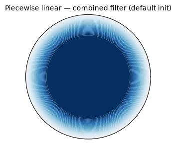
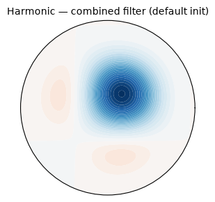
    # combined filter with default init
    filt = (fb.get_init_factors().reshape(-1, 1, 1) * psi).sum(dim=0)
    fig, ax = plt.subplots(figsize=(3, 3), subplot_kw={"projection": "polar"})
    vmax = filt.abs().max().item() or 1.0
    ax.contourf(phi, r, filt, cmap=cmap, vmin=-vmax, vmax=vmax,
                levels=24, antialiased=True)
    ax.set_title(f"{title} — combined filter (default init)", fontsize=10)
    ax.set_xticks([])
    ax.set_yticks([])
    plt.tight_layout()
    plt.show()

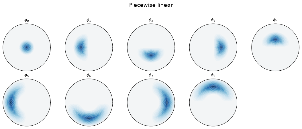
3.1 Piecewise linear

The simplest basis: tensor-product hat functions on a polar grid with n_radial radial rings and n_angular angular sectors. Each basis function is non-zero on a single cell of the polar grid and interpolates linearly. This is analogous to bilinear elements in finite element methods.

fb_pwl = get_filter_basis((5, 4), "piecewise linear")
print(f"kernel_shape=(5, 4)  =>  K = {fb_pwl.kernel_size} basis functions")
plot_basis(fb_pwl, "Piecewise linear")

kernel_shape=(5, 4)  =>  K = 9 basis functions

3.2 Harmonic (Hann-windowed Fourier)

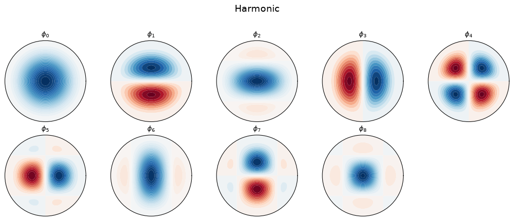
A smooth basis using Hann-windowed sinusoidal modes in the radial direction and Fourier modes in the angular direction. The Hann window ensures the basis functions decay smoothly to zero at the boundary, avoiding discontinuities. The basis functions are L2-normalised on the unit disk.

fb_har = get_filter_basis((3, 3), "harmonic")
print(f"kernel_shape=(3, 3)  =>  K = {fb_har.kernel_size} basis functions")
plot_basis(fb_har, "Harmonic")

kernel_shape=(3, 3)  =>  K = 9 basis functions

3.3 Zernike polynomials

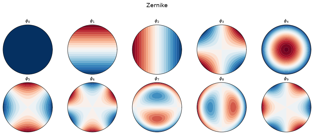
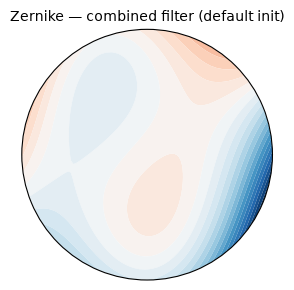
The Zernike polynomials form an orthogonal basis on the unit disk. They are widely used in optics and wavefront analysis. kernel_shape is a single integer n_max controlling the maximum radial degree; the total number of basis functions is \(\tfrac{1}{2}(n_{\max}+1)(n_{\max}+2)\).

fb_zer = get_filter_basis(4, "zernike")
print(f"kernel_shape=4  =>  K = {fb_zer.kernel_size} basis functions")
plot_basis(fb_zer, "Zernike")

kernel_shape=4  =>  K = 10 basis functions

3.4 Fourier–Bessel

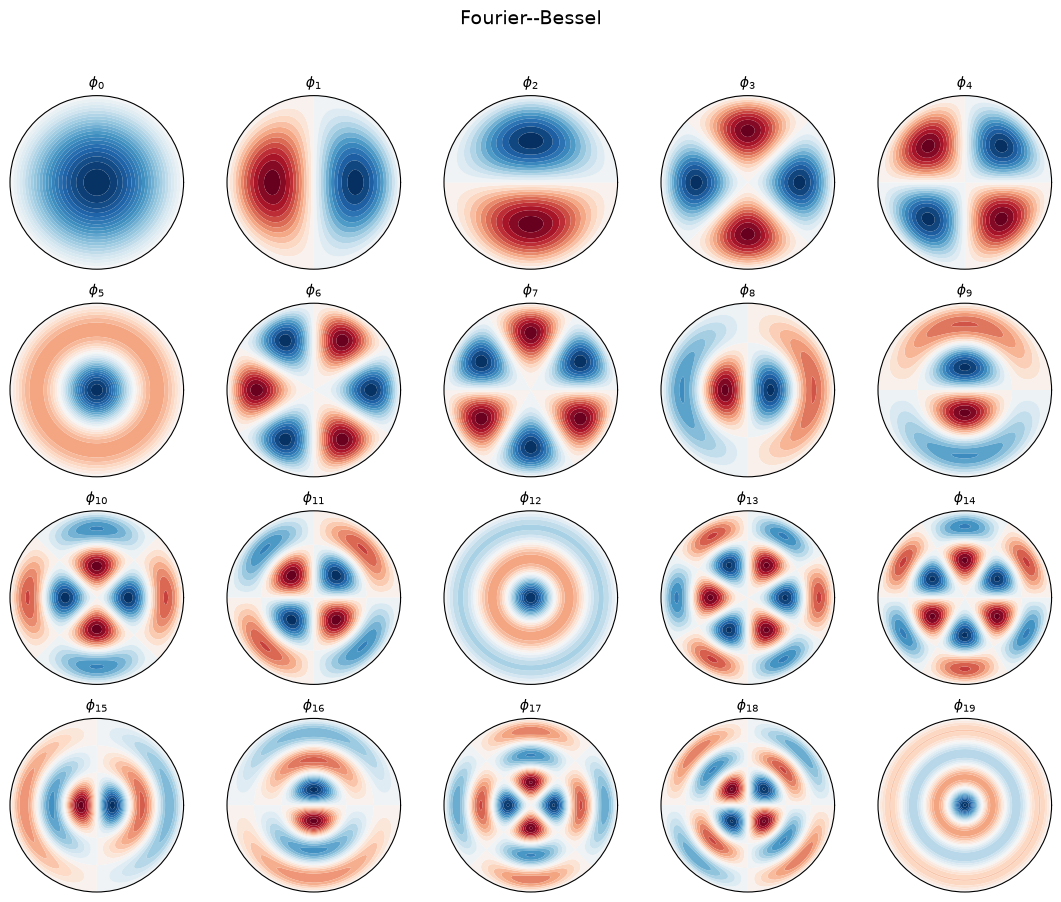
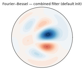
The Fourier–Bessel basis functions on a disk are defined as

\[ \Psi_{m,n}(r, \varphi) = J_m(\alpha_{m,n}\,r)\,\cos(m\,\varphi) \]

where \(J_m\) is the Bessel function of the first kind and \(\alpha_{m,n}\) is its \(n\)-th positive zero. Unlike the Zernike polynomials, these basis functions vanish at the boundary of the disk (\(r = 1\)), which avoids edge artefacts in the convolution.

Note

This basis requires SciPy to be installed.

fb_fbs = get_filter_basis((4, 3), "fourier-bessel")
print(f"kernel_shape=(4, 3)  =>  K = {fb_fbs.kernel_size} basis functions")
plot_basis(fb_fbs, "Fourier--Bessel")

kernel_shape=(4, 3)  =>  K = 20 basis functions

4. Running a DISCO convolution

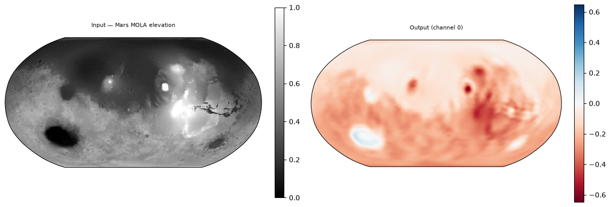
With the mathematical background in place, let’s run a concrete convolution. We use the MOLA digital elevation map of Mars (courtesy of NASA) as a realistic input signal on the sphere and apply a DiscreteContinuousConvS2 layer.

import torch.nn.functional as F

import torch_harmonics as th
from torch_harmonics.utils import load_mola_elevation

nlat, nlon = 128, 256
signal = load_mola_elevation(nlat, nlon).unsqueeze(0).unsqueeze(0)

in_channels, out_channels = 1, 8

torch.manual_seed(333)

conv = th.DiscreteContinuousConvS2(
    in_channels=in_channels,
    out_channels=out_channels,
    in_shape=(nlat, nlon),
    out_shape=(nlat, nlon),
    kernel_shape=(5, 4),
    basis_type="piecewise linear",
    theta_cutoff=0.2,
)

y = conv(signal)

print(f"Input shape:  {signal.shape}")
print(f"Output shape: {y.shape}")

Input shape:  torch.Size([1, 1, 128, 256])
Output shape: torch.Size([1, 8, 128, 256])

Let’s visualise the input and one output channel:

fig = plt.figure(figsize=(12, 4), layout="constrained")
subfigs = fig.subfigures(1, 2)

plot_sphere(signal[0, 0].detach(), fig=subfigs[0], cmap="gray",
            title="Input — Mars MOLA elevation", colorbar=True)

vmax = y[0, 0].abs().max().item()
plot_sphere(y[0, 0].detach(), fig=subfigs[1], cmap="RdBu",
            title="Output (channel 0)", colorbar=True,
            vmin=-vmax, vmax=vmax)

plt.show()

5. The \(\Psi\) tensor in practice

The precomputed \(\Psi\) tensor is stored in COO sparse format on the module. Let’s inspect its sparsity and how it scales with resolution and theta_cutoff.

# sparsity at different resolutions
for nlat, nlon in [(32, 64), (64, 128), (128, 256)]:
    conv_res = th.DiscreteContinuousConvS2(
        in_channels=1, out_channels=1,
        in_shape=(nlat, nlon), out_shape=(nlat, nlon),
        kernel_shape=(5, 4), basis_type="piecewise linear",
    )
    nnz = conv_res.psi_vals.numel()
    total = conv_res.kernel_size * nlat * nlat * nlon
    print(f"Grid {nlat:3d}x{nlon:3d}: "
          f"{nnz:>8,} nonzeros in Psi "
          f"(density {100*nnz/total:.3f}%)")

Grid  32x 64:    1,689 nonzeros in Psi (density 0.286%)
Grid  64x128:    3,549 nonzeros in Psi (density 0.075%)
Grid 128x256:    7,481 nonzeros in Psi (density 0.020%)

# effect of theta_cutoff on the number of nonzeros
nlat, nlon = 64, 128
for tc in [0.05, 0.1, 0.2, 0.4]:
    conv_tc = th.DiscreteContinuousConvS2(
        in_channels=1, out_channels=1,
        in_shape=(nlat, nlon), out_shape=(nlat, nlon),
        kernel_shape=(5, 4), basis_type="piecewise linear",
        theta_cutoff=tc,
    )
    nnz = conv_tc.psi_vals.numel()
    print(f"theta_cutoff={tc:.2f} rad ({math.degrees(tc):5.1f} deg): "
          f"{nnz:>8,} nonzeros")

theta_cutoff=0.05 rad (  2.9 deg):    3,565 nonzeros
theta_cutoff=0.10 rad (  5.7 deg):   10,653 nonzeros
theta_cutoff=0.20 rad ( 11.5 deg):   29,228 nonzeros
theta_cutoff=0.40 rad ( 22.9 deg):   92,846 nonzeros

6. Choosing theta_cutoff and kernel_shape

These are the two main hyperparameters:

• theta_cutoff controls how far each output point can “see” on the sphere. A larger cutoff increases the receptive field but also increases the number of nonzeros in \(\Psi\) (and thus cost and memory). If not specified, it defaults to \(\pi / (N_{\text{lat,out}} - 1)\), which is roughly one grid spacing.

• kernel_shape controls the number of learnable degrees of freedom per channel pair. More basis functions allow the filter to represent more complex spatial patterns, but increase the parameter count.

The interplay between the two matters: a large theta_cutoff with too few basis functions undersamples the filter, while many basis functions crammed into a tiny support are wasteful.

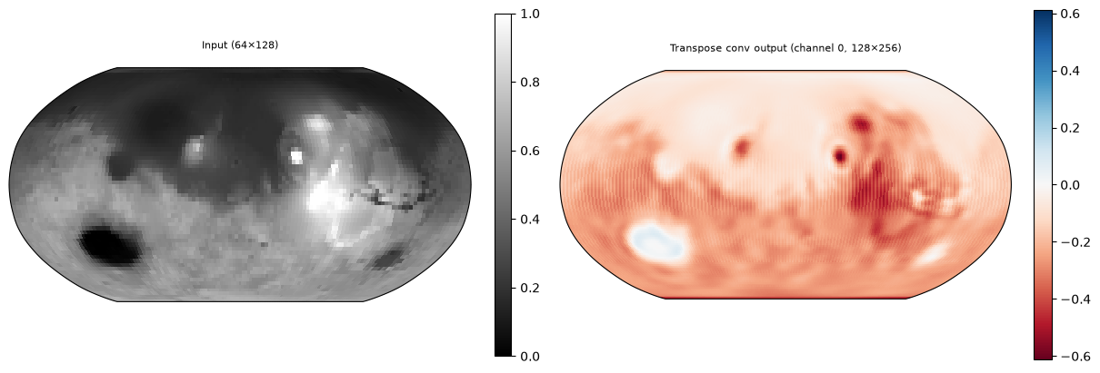
7. Transpose convolution

DiscreteContinuousConvTransposeS2 applies the \(\Psi\) tensor in the reverse direction, mapping a coarser grid to a finer one (upsampling). It uses the same filter basis and compact-support construction. This is the adjoint of the forward convolution and is typically used in decoder / upsampling paths of U-Net-style architectures on the sphere.

nlat_coarse, nlon_coarse = 64, 128
nlat_fine, nlon_fine = 128, 256

signal_coarse = F.interpolate(signal, size=(nlat_coarse, nlon_coarse),
                              mode="bilinear", align_corners=False)

torch.manual_seed(333)

conv_up = th.DiscreteContinuousConvTransposeS2(
    in_channels=1, out_channels=8,
    in_shape=(nlat_coarse, nlon_coarse),
    out_shape=(nlat_fine, nlon_fine),
    kernel_shape=(5, 4),
    basis_type="piecewise linear",
    theta_cutoff=0.2,
)

y_up = conv_up(signal_coarse)
print(f"Input:  {signal_coarse.shape}")
print(f"Output: {y_up.shape}")

Input:  torch.Size([1, 1, 64, 128])
Output: torch.Size([1, 8, 128, 256])

fig = plt.figure(figsize=(12, 4), layout="constrained")
subfigs = fig.subfigures(1, 2)

plot_sphere(signal_coarse[0, 0].detach(), fig=subfigs[0], cmap="gray",
            title=f"Input ({nlat_coarse}×{nlon_coarse})", colorbar=True)

vmax = y_up[0, 0].abs().max().item()
plot_sphere(y_up[0, 0].detach(), fig=subfigs[1], cmap="RdBu",
            title=f"Transpose conv output (channel 0, {nlat_fine}×{nlon_fine})",
            colorbar=True, vmin=-vmax, vmax=vmax)

plt.show()

Summary

• DISCO convolutions combine a continuous filter (learnable weights over basis functions) with discrete quadrature to achieve \(O(N)\) spherical convolutions with approximate \(SO(3)\) equivariance.

• The precomputed \(\Psi\) tensor is sparse (compact support) and longitude-invariant (p-shift), making the convolution efficient.

• Four basis types are available: piecewise linear, harmonic, Zernike, and Fourier–Bessel. The choice affects the smoothness and expressiveness of the filter.

• theta_cutoff and kernel_shape are the key hyperparameters controlling receptive field and filter complexity.

Tip

When running on CPU, the DISCO convolution kernels are parallelised with OpenMP. Setting OMP_NUM_THREADS to the number of physical cores can significantly improve performance. The optimal thread binding depends on your hardware:

• OMP_PROC_BIND=close packs threads onto adjacent cores, which is usually best on single-socket machines where threads benefit from shared cache.

• OMP_PROC_BIND=spread distributes threads across sockets or chiplets, which can be better on multi-socket or AMD EPYC systems where aggregate memory bandwidth is the bottleneck.

For Intel OpenMP, the equivalent settings are KMP_AFFINITY=compact and KMP_AFFINITY=scatter.

export OMP_NUM_THREADS=8
export OMP_PROC_BIND=close   # or spread on multi-socket systems

For the full parameter documentation, see the DiscreteContinuousConvS2 and DiscreteContinuousConvTransposeS2 API pages.