Spectral convolutions on the sphere

This guide explains the spectral convolution layer SpectralConvS2. Unlike the DISCO convolution (which operates in the spatial domain with compact-support kernels), the spectral convolution works entirely in the spherical harmonic domain, making it naturally isotropic (azimuthally symmetric) and global in receptive field.

1. Convolution via the spectral theorem

On the sphere, convolution with an isotropic (axisymmetric) kernel is diagonal in the spherical harmonic basis. This is the spherical analogue of the classical convolution theorem on \(\mathbb{R}^n\): convolution in the spatial domain corresponds to pointwise multiplication in the spectral domain.

Given a multi-channel input \(u^{c_i}(\theta, \lambda)\), the spectral convolution computes output channels \(v^{c_o}(\theta, \lambda)\) in three steps:

1. Forward SHT — transform each input channel to spectral space:

\[ \hat{u}_l^{m,\,c_i} = \text{SHT}\!\left[\, u^{c_i}(\theta, \lambda) \,\right] \]

2. Spectral contraction — mix channels with learnable weights \(K_l^{c_o,\,c_i}\) that depend only on degree \(l\) (not order \(m\)):

\[ \hat{v}_l^{m,\,c_o} = \sum_{c_i} K_l^{c_o,\,c_i}\; \hat{u}_l^{m,\,c_i} \]

3. Inverse SHT — transform back to the spatial domain:

\[ v^{c_o}(\theta, \lambda) = \text{ISHT}\!\left[\, \hat{v}_l^{m,\,c_o} \,\right] \]

Because the weights depend only on degree \(l\) and not on order \(m\), this corresponds to an isotropic convolution kernel on the sphere — the filter response is the same in every direction.

2. Spectral vs. spatial convolution

	Spectral (SpectralConvS2)	Spatial (DiscreteContinuousConvS2)
Domain	Spherical harmonic (frequency)	Spatial (grid points)
Kernel symmetry	Isotropic (axisymmetric)	Anisotropic (arbitrary azimuthal dependence)
Receptive field	Global (all degrees up to \(l_{\max}\))	Local (compact support within \(\theta_{\text{cutoff}}\))
Cost	\(\mathcal{O}(N \log N)\) (FFT) + \(\mathcal{O}(N l_{\max})\) (Legendre)	\(\mathcal{O}(kN)\) (sparse, \(k\) = neighbors)
Parameters per channel pair	\(l_{\max}\) complex weights	\(K\) real weights (basis functions)
Resolution agnostic	Yes (truncate or zero-pad spectrum)	Yes (re-evaluate \(\Psi\) on new grid)

The spectral convolution is a natural choice when the filter should be rotationally symmetric (e.g. diffusion, smoothing, spectral filtering). When the filter needs azimuthal structure (e.g. edge detection, directional features), the DISCO convolution is more expressive.

3. Spectral bias

When bias=True, a learnable spectral bias \(b_l^{m,\,c_i}\) is added to the SHT coefficients before the channel contraction. The bias is modulated by the spatial integral (zeroth moment) of each input channel:

\[ I^{c_i} = \int_0^{2\pi}\!\int_0^{\pi} u^{c_i}(\theta,\lambda)\,\sin\theta\;d\theta\;d\lambda \]

\[ \hat{u}_l^{m,\,c_i} \;\leftarrow\; \hat{u}_l^{m,\,c_i} + I^{c_i}\, b_l^{m,\,c_i} \]

This couples the global mean of each input channel into all spectral modes, allowing the layer to learn a spectral response that depends on the overall signal level.

4. Example: spectral convolution on Mars elevation

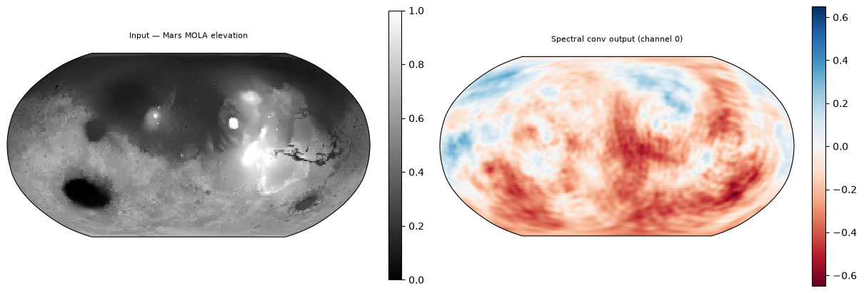
Let’s apply a spectral convolution to the Mars MOLA elevation map and inspect the output. Because the convolution is isotropic, each output channel is a rotationally symmetric filtering of the input — similar to applying a radial low-pass or band-pass filter.

import matplotlib.pyplot as plt
import torch
import torch.nn.functional as F

import torch_harmonics as th
from torch_harmonics.plotting import plot_sphere
from torch_harmonics.utils import load_mola_elevation

nlat, nlon = 128, 256
signal = load_mola_elevation(nlat, nlon).unsqueeze(0).unsqueeze(0)

in_channels, out_channels = 1, 8

torch.manual_seed(333)

spec_conv = th.SpectralConvS2(
    in_shape=(nlat, nlon),
    out_shape=(nlat, nlon),
    in_channels=in_channels,
    out_channels=out_channels,
)

y = spec_conv(signal)

print(f"Input shape:  {signal.shape}")
print(f"Output shape: {y.shape}")
print(f"Spectral weights shape: {spec_conv.weight.shape}")
print("  (num_groups, in_channels/groups, out_channels/groups, lmax)")
print(f"lmax = {spec_conv.lmax}")

/opt/anaconda/envs/torch-harmonics/lib/python3.12/site-packages/torch_harmonics/truncation.py:168: UserWarning: Default SHT truncation changed in v0.9.0: equiangular/equiangular-trapezoidal grids now truncate to (nlat+1)//2. Specify lmax explicitly to override.
  lmax = lmax or _truncate_lmax(nlat, grid)

Input shape:  torch.Size([1, 1, 128, 256])
Output shape: torch.Size([1, 8, 128, 256])
Spectral weights shape: torch.Size([1, 1, 8, 64])
  (num_groups, in_channels/groups, out_channels/groups, lmax)
lmax = 64

/opt/anaconda/envs/torch-harmonics/lib/python3.12/site-packages/torch/_inductor/lowering.py:2633: UserWarning: Torchinductor does not support code generation for complex operators. Performance may be worse than eager.
  warnings.warn(

fig = plt.figure(figsize=(12, 4), layout="constrained")
subfigs = fig.subfigures(1, 2)

plot_sphere(signal[0, 0].detach(), fig=subfigs[0], cmap="gray",
            title="Input — Mars MOLA elevation", colorbar=True)

vmax = y[0, 0].abs().max().item()
plot_sphere(y[0, 0].detach(), fig=subfigs[1], cmap="RdBu",
            title="Spectral conv output (channel 0)", colorbar=True,
            vmin=-vmax, vmax=vmax)

plt.show()

5. Visualising the spectral weights

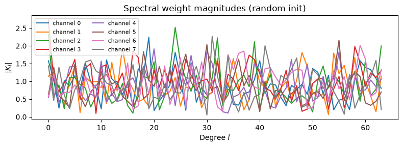
Each output channel has a weight vector of length \(l_{\max}\) that controls how strongly each spherical harmonic degree contributes. Let’s plot the magnitude of the spectral weights for all output channels.

fig, ax = plt.subplots(figsize=(8, 3))

# weight shape: (num_groups, in_ch/groups, out_ch/groups, lmax)
w = spec_conv.weight.detach()
for c in range(out_channels):
    ax.plot(w[0, 0, c].abs().numpy(), label=f"channel {c}")

ax.set_xlabel("Degree $l$")
ax.set_ylabel("$|K_l|$")
ax.set_title("Spectral weight magnitudes (random init)")
ax.legend(fontsize=8, ncol=2)
plt.tight_layout()
plt.show()

6. Grouped spectral convolution

Like grouped convolutions in CNNs, setting num_groups > 1 partitions the input and output channels into independent groups. Each group has its own spectral weights, reducing the parameter count from \(l_{\max} \times C_{\text{in}} \times C_{\text{out}}\) to \(l_{\max} \times C_{\text{in}} \times C_{\text{out}} / G\) where \(G\) is the number of groups.

in_ch, out_ch = 16, 32

for ng in [1, 4, 16]:
    torch.manual_seed(333)
    sc = th.SpectralConvS2(
        in_shape=(nlat, nlon),
        out_shape=(nlat, nlon),
        in_channels=in_ch,
        out_channels=out_ch,
        num_groups=ng,
    )
    nparams = sum(p.numel() for p in sc.parameters())
    print(f"num_groups={ng:2d}: weight shape {tuple(sc.weight.shape)}, "
          f"total params = {nparams:,}")

num_groups= 1: weight shape (1, 16, 32, 64), total params = 32,768
num_groups= 4: weight shape (4, 4, 8, 64), total params = 8,192
num_groups=16: weight shape (16, 1, 2, 64), total params = 2,048

/opt/anaconda/envs/torch-harmonics/lib/python3.12/site-packages/torch_harmonics/truncation.py:168: UserWarning: Default SHT truncation changed in v0.9.0: equiangular/equiangular-trapezoidal grids now truncate to (nlat+1)//2. Specify lmax explicitly to override.
  lmax = lmax or _truncate_lmax(nlat, grid)

7. Resolution transfer

Because the learnable weights live in spectral space, the same weights can be applied on a different grid resolution — just change in_shape and out_shape. If the new grid has a lower resolution, the spectrum is truncated to the smaller \(l_{\max}\); if higher, the extra modes are simply absent from the weight tensor (equivalent to zero-padding in frequency).

for res in [(64, 128), (128, 256), (256, 512)]:
    torch.manual_seed(333)
    sc = th.SpectralConvS2(
        in_shape=res,
        out_shape=res,
        in_channels=1,
        out_channels=8,
    )
    print(f"Grid {res[0]:3d}×{res[1]:3d}: lmax = {sc.lmax}, "
          f"weight shape {tuple(sc.weight.shape)}")

Grid  64×128: lmax = 32, weight shape (1, 1, 8, 32)
Grid 128×256: lmax = 64, weight shape (1, 1, 8, 64)
Grid 256×512: lmax = 128, weight shape (1, 1, 8, 128)

8. Up- and downsampling

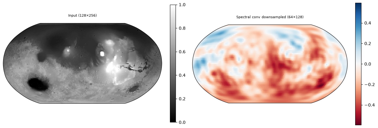
The input and output grids do not need to match. Setting a coarser out_shape naturally downsamples through spectral truncation, while a finer out_shape upsamples by synthesising back onto a denser grid.

torch.manual_seed(333)

# downsample: 128x256 -> 64x128
spec_down = th.SpectralConvS2(
    in_shape=(128, 256),
    out_shape=(64, 128),
    in_channels=1,
    out_channels=1,
)

# upsample: 64x128 -> 128x256
spec_up = th.SpectralConvS2(
    in_shape=(64, 128),
    out_shape=(128, 256),
    in_channels=1,
    out_channels=1,
)

y_down = spec_down(signal)
y_up = spec_up(F.interpolate(signal, size=(64, 128), mode="bilinear", align_corners=False))

print(f"Input:       {signal.shape}")
print(f"Downsampled: {y_down.shape}")
print(f"Upsampled:   {y_up.shape}")

Input:       torch.Size([1, 1, 128, 256])
Downsampled: torch.Size([1, 1, 64, 128])
Upsampled:   torch.Size([1, 1, 128, 256])

fig = plt.figure(figsize=(12, 4), layout="constrained")
subfigs = fig.subfigures(1, 2)

plot_sphere(signal[0, 0].detach(), fig=subfigs[0], cmap="gray",
            title="Input (128×256)", colorbar=True)

vmax = y_down[0, 0].abs().max().item()
plot_sphere(y_down[0, 0].detach(), fig=subfigs[1], cmap="RdBu",
            title="Spectral conv downsampled (64×128)", colorbar=True,
            vmin=-vmax, vmax=vmax)

plt.show()

Summary

• Spectral convolution implements convolution on \(S^2\) by pointwise multiplication in the spherical harmonic domain (SHT \(\to\) spectral contraction \(\to\) inverse SHT).

• The spectral weights depend only on degree \(l\), making the kernel isotropic with a global receptive field.

• An optional spectral bias couples the spatial mean of each channel into all spectral modes.

• Grouped convolution reduces parameters by partitioning channels.

• The layer is resolution-agnostic: the same weights can be evaluated on different grids, and mismatched input/output shapes naturally up- or downsample.

For the full parameter documentation, see SpectralConvS2.