Stanford 2D-3D-S dataset

The Stanford 2D-3D-Semantics dataset provides panoramic RGB images of indoor scenes together with per-pixel semantic labels and depth maps. Because each panorama covers a full 360° field of view, the images live naturally on the 2-sphere — making them an ideal benchmark for spherical neural networks.

This notebook shows how to:

1. Download and prepare the dataset using Stanford2D3DSDownloader

2. Visualize RGB inputs, semantic segmentation labels, and depth maps

3. Inspect the class distribution and depth statistics

Setup

import os
import numpy as np
import h5py as h5

import matplotlib as mpl
import matplotlib.pyplot as plt
import matplotlib.patches as mpatches

from torch_harmonics.plotting import imshow_sphere, plot_sphere

from torch_harmonics.examples import Stanford2D3DSDownloader

/home/thorsten/.conda/envs/torch_harmonics/lib/python3.12/site-packages/torch/cuda/__init__.py:63: FutureWarning: The pynvml package is deprecated. Please install nvidia-ml-py instead. If you did not install pynvml directly, please report this to the maintainers of the package that installed pynvml for you.
  import pynvml  # type: ignore[import]

Download and prepare the dataset

The Stanford2D3DSDownloader handles downloading, extracting, and converting the raw panoramas into an HDF5 file. If the file already exists the download is skipped:

data_dir = "../examples/data/2D3DS"
os.makedirs(data_dir, exist_ok=True)

# 2D3DS download & dataset initialization
downloader = Stanford2D3DSDownloader(base_url="https://cvg-data.inf.ethz.ch/2d3ds/no_xyz/", local_dir=str(data_dir))
dataset_file = downloader.prepare_dataset([("area_1_no_xyz.tar", "area_1")], "stanford_2d3ds_dataset_ds16.h5")

Dataset file at ../examples/data/2D3DS/stanford_2d3ds_dataset_ds16.h5 already exists. Skipping download and conversion. If you want to create a new dataset file, delete or rename the existing file.

Loading the dataset

The HDF5 file contains the RGB images, semantic labels, depth maps, and associated metadata (class labels, normalization statistics). We load a single sample to inspect:

h5file = h5.File(dataset_file, "r")

inp = np.transpose(h5file["rgb"][0, ...], (1,2,0))
tar = h5file["semantic"][0, ...]
dep = h5file["depth"][0, ...]
class_labels = h5file["class_labels"]
class_histogram = h5file["class_histogram"]
num_classes = len(class_labels)

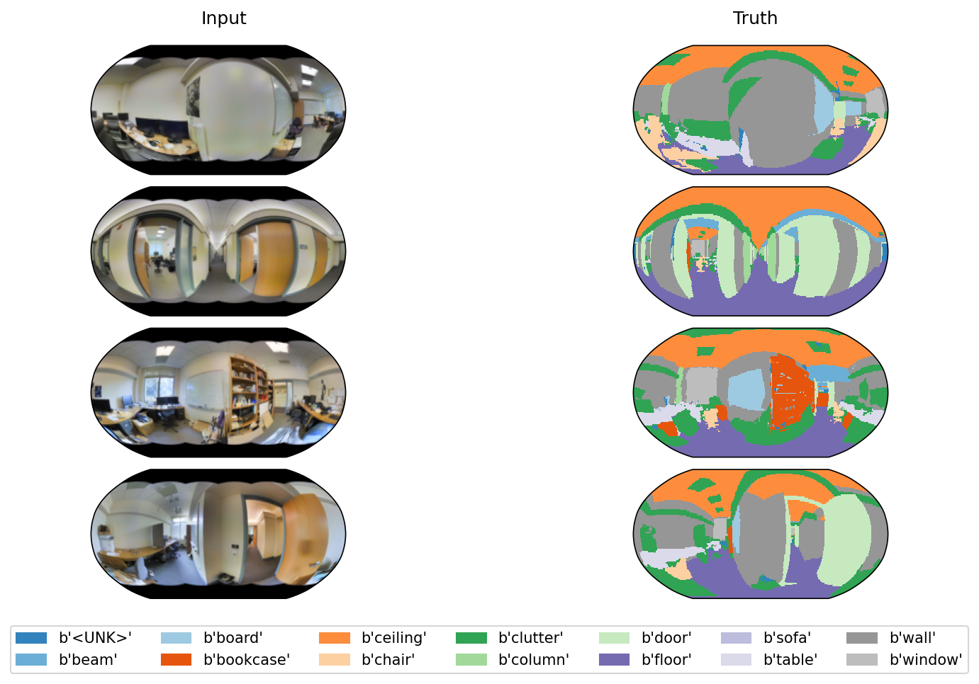
Semantic segmentation

Each pixel is assigned one of 14 semantic classes (wall, floor, ceiling, furniture, etc.). Let us visualize a few samples side-by-side with their RGB inputs. The class labels stored in the dataset are:

class_labels

<HDF5 dataset "class_labels": shape (14,), type "|O">

num_samples = 4

fig = plt.figure(layout="constrained", figsize=(10, 6.5), dpi=150)

# thin strips at the top (column headers) and bottom (legend) so every image
# row keeps the same size -- putting titles inside the top-row subfigures would
# shrink only the first row.
header_fig, grid_fig, legend_fig = fig.subfigures(
    3, 1, height_ratios=[0.25, num_samples, 0.6]
)

# 2 columns (Input, Truth)
subfigs = grid_fig.subfigures(num_samples, 2, wspace=0.04)

cmap = mpl.colormaps["tab20c"]

for isample in range(num_samples):

    inp = np.transpose(h5file["rgb"][isample, ...], (1, 2, 0))
    tar = h5file["semantic"][isample, ...]

    # do the plotting
    imshow_sphere(inp, fig=subfigs[isample, 0])
    plot_sphere(tar / num_classes, fig=subfigs[isample, 1], cmap=cmap, vmin=0.0, vmax=1.0)

# build the legend handles once
legend_list = [
    mpatches.Patch(color=cmap(cidx / num_classes), label=cname)
    for cidx, cname in enumerate(class_labels)
]

# column headers in their own top strip (aligned with the two columns)
for j, label in enumerate(["Input", "Truth"]):
    header_fig.text((j + 0.5) / 2, 0.5, label, va="center", ha="center", fontsize="large")

# legend in its own bottom strip
legend_fig.legend(handles=legend_list, loc="center", ncol=7)

<matplotlib.legend.Legend at 0x7efab0a61a00>

Class distribution

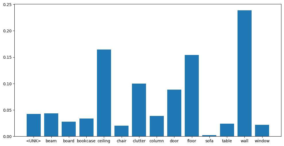
The class histogram reveals a strong imbalance — walls, floors, and ceilings dominate, while objects like boards and bookcases are rare. This imbalance is important to account for when training segmentation models:

class_labels = [cl.decode("utf-8") for cl in class_labels]

fig = plt.figure(figsize=(12,6))
plt.bar(class_labels, class_histogram)
plt.show()

Depth estimation

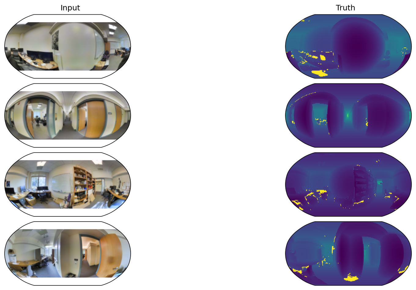
The dataset also provides per-pixel depth maps and validity masks. We visualize the log-depth (to compress the dynamic range) alongside the RGB input. Poles are masked white since the equirectangular projection is degenerate there:

num_samples = 4

fig = plt.figure(figsize=(12, 6), dpi=150, layout="constrained")
subfigs = fig.subfigures(num_samples, 2, wspace=0.04)

cmap = mpl.colormaps["tab20c"]

for isample in range(num_samples):

    inp = np.transpose(h5file["rgb"][isample, ...], (1,2,0))
    inp[0:20, :, :] = [1, 1, 1]
    inp[-20:, :, :] = [1, 1, 1]
    tar = h5file["depth"][isample, ...]
    # depth_mask is not stored in the dataset -- invalid pixels are encoded as the
    # maximum depth value, so derive the mask on the fly (cf. Depth._mask_invalid)
    mask = np.where(tar == tar.max(), 0, 1)

    # do the plotting
    imshow_sphere(inp, fig=subfigs[isample, 0])
    imshow_sphere(np.log(tar)*mask, fig =subfigs[isample, 1], cmap="viridis")

# Add column labels
column_labels = ["Input", "Truth"]
for j, label in enumerate(column_labels):
    fig.text((j + 0.5) / 2, 1.03, label, va="top", ha="center", fontsize="large")

Depth statistics

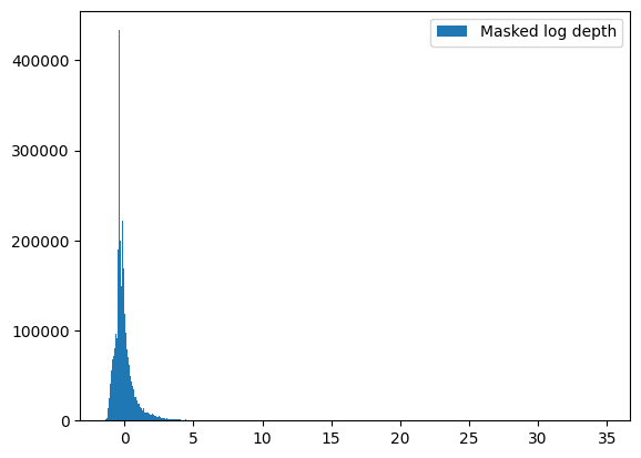
We compute the distribution of log-depth values across the dataset. The normalization statistics (mean, std) stored in the HDF5 file can be used for standardizing the depth targets during training:

min_depth = h5file["min_depth"][...]
max_depth = h5file["max_depth"][...]
mean_depth = h5file["mean_depth"][...]
std_depth = h5file["std_depth"][...]

depth = h5file["depth"][...]
# invalid pixels are encoded as the maximum depth value (no stored mask)
mask_depth = np.where(depth == depth.max(), 0, 1)

print("Max: ", depth.max())
print("Min: ", depth.min())
m = np.log(1 + depth) * mask_depth
m = m[m!=0]
print(f"Mean log depth: {np.nanmean(m)}")
print(f"Std log depth: {np.nanstd(m)}")
m = (m - np.mean(m)) / np.std(m)

counts, bin_edges, _ = plt.hist(m.flatten(), 1000, label="Masked log depth")
plt.legend()

Max:  0.99998474
Min:  0.0016479492
Mean log depth: 0.01472963752582171
Std log depth: 0.009298770923114956

<matplotlib.legend.Legend at 0x7efab0564ec0>

RGB statistics

Per-channel RGB statistics for input normalization:

min_rgb = h5file["min_rgb"][...]
max_rgb = h5file["max_rgb"][...]
mean_rgb = h5file["mean_rgb"][...]
std_rgb = h5file["std_rgb"][...]

print(f"Min rgb: {min_rgb}")
print(f"Max rgb: {max_rgb}")
print(f"Mean rgb: {mean_rgb}")
print(f"Std rgb: {std_rgb}")

Min rgb: [0. 0. 0.]
Max rgb: [0.84705883 0.8        0.81960785]
Mean rgb: [0.49967027 0.48454845 0.4377965 ]
Std rgb: [0.38496047 0.38471302 0.38496676]