Helmholtz equation

This notebook demonstrates a differentiable spectral solver for reaction–diffusion equations on the sphere, built on torch-harmonics. The solver supports two PDEs:

• Allen–Cahn: \(\partial_t u = \epsilon\,\Delta u + u - u^3\)

• Ginzburg–Landau: \(\partial_t u = \epsilon\,\Delta u + u - (1+i\beta)\,|u|^2 u\)

Time integration is performed in spectral space using third-order Adams–Bashforth, and the results are saved as an animated GIF.

Setup

import torch
import matplotlib.pyplot as plt
import matplotlib.animation as animation

from math import ceil
from tqdm.auto import tqdm

from torch_harmonics.examples import SphereSolver

cmap='twilight_shifted'

/opt/anaconda/envs/torch-harmonics/lib/python3.12/site-packages/tqdm/auto.py:21: TqdmWarning: IProgress not found. Please update jupyter and ipywidgets. See https://ipywidgets.readthedocs.io/en/stable/user_install.html
  from .autonotebook import tqdm as notebook_tqdm

device = torch.device('cuda' if torch.cuda.is_available() else 'cpu')

Solver configuration

The SphereSolver class provides the spectral infrastructure: it precomputes the SHT operators, quadrature weights, and the hyperdiffusion filter. We choose a resolution of 128 latitudes, a diffusion coefficient of 0.01, and integrate for 10 time units with \(\Delta t = 0.001\).

# initialize parameters:
nlat = 128
nlon = 2*nlat
lmax = ceil(nlon/4)
mmax = lmax

# timestepping
dt = 0.001
maxiter = int(10 / dt)

# initialize solver class
solver = SphereSolver(nlat, nlon, dt, lmax=lmax, mmax=mmax, coeff=0.01).to(device)

lons = solver.lons
lats = solver.lats

jj, ii = torch.triu_indices(lmax, mmax)

Initial condition

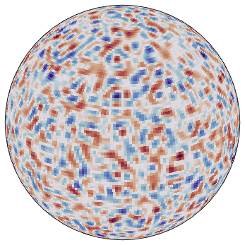
We generate a random initial condition in spectral space using solver.randspec(). This produces a band-limited random field on the sphere:

uspec0 = solver.randspec()
fig = plt.figure(figsize=(8, 6), dpi=72)
solver.plot_specdata(uspec0, fig, cmap=cmap)
plt.show()

Time integration

We integrate the PDE using third-order Adams–Bashforth. Every 20 steps, the current state is rendered into the animation. Since we only need the forward pass, the loop runs inside torch.no_grad() to save memory.

import os
os.makedirs("plots", exist_ok=True)

dudtspec = torch.zeros(3, solver.lmax, solver.mmax, dtype=torch.complex128, device=device)
nnew = 0
nnow = 1
nold = 2

uspec = uspec0.clone().to(device)
# pde = 'allen-cahn'
pde = 'ginzburg-landau'


# prepare figure for animation
fig = plt.figure(figsize=(8, 6), dpi=72)
moviewriter = animation.writers['pillow'](fps=20)
moviewriter.setup(fig, f'./plots/{pde}.gif', dpi=72)


pbar = tqdm(range(maxiter+1), desc="Helmholtz integration")
with torch.no_grad():
    for iter in pbar:
        t = iter*dt

        if iter % 20 == 0:
            pbar.set_postfix_str(f"t={t:.2f}")
            plt.clf()
            solver.plot_specdata(uspec, fig, cmap=cmap)
            plt.draw()
            moviewriter.grab_frame()

        dudtspec[nnew] = solver.dudtspec(uspec, pde=pde)
        
        # forward euler, then 2nd-order adams-bashforth time steps to start.
        if iter == 0:
            dudtspec[nnow] = dudtspec[nnew]
            dudtspec[nold] = dudtspec[nnew]
        elif iter == 1:
            dudtspec[nold] = dudtspec[nnew]

        uspec = uspec + solver.dt*( (23./12.) * dudtspec[nnew] - (16./12.) * dudtspec[nnow] + (5./12.) * dudtspec[nold] )

        # cycle through the indices
        nsav1 = nnew
        nsav2 = nnow
        nnew = nold
        nnow = nsav1
        nold = nsav2


moviewriter.finish()

Helmholtz integration: 100%|██████████| 10001/10001 [00:23<00:00, 417.34it/s, t=10.00]