Getting started with `torch-harmonics`#

This notebook walks through the basic usage of the torch-harmonics library:

Forward and inverse SHT — compute spectral coefficients from grid data and reconstruct
Visualization — inspect spectral coefficients and round-trip reconstruction error
Differentiability — fit spectral coefficients to a target signal using gradient descent

Usage#

Preparation#

Let us begin by loading some libraries that we will be needing:

import torch
import torch.nn as nn
import matplotlib.pyplot as plt

from tqdm.auto import tqdm

from torch_harmonics import RealSHT, InverseRealSHT
from torch_harmonics.plotting import plot_sphere
from torch_harmonics.utils import load_mola_elevation

cmap = "turbo"

Test data#

We use the MOLA digital elevation map of Mars (courtesy of NASA) as test data. The helper function downloads and caches the image automatically:

nlat, nlon = 512, 1024
data = load_mola_elevation(nlat, nlon)

Spherical harmonic transform#

torch_harmonics provides the forward and inverse SHT as standard PyTorch modules (RealSHT and InverseRealSHT). This means they can be moved to the GPU with .to(device), composed with other modules, and differentiated through with autograd.

device = torch.device('cuda' if torch.cuda.is_available() else 'cpu')

signal = data.to(device)

sht = RealSHT(nlat, nlon, grid="equiangular").to(device)
isht = InverseRealSHT(nlat, nlon, grid="equiangular").to(device)

/opt/anaconda/envs/torch-harmonics/lib/python3.12/site-packages/torch_harmonics/truncation.py:168: UserWarning: Default SHT truncation changed in v0.9.0: equiangular/equiangular-trapezoidal grids now truncate to (nlat+1)//2. Specify lmax explicitly to override.
  lmax = lmax or _truncate_lmax(nlat, grid)

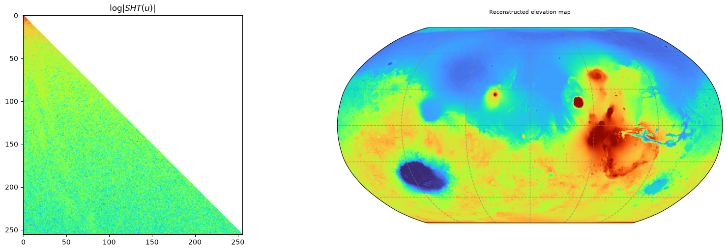
The forward SHT projects the grid data onto the spherical harmonic basis functions, yielding complex-valued spectral coefficients \(\hat{u}_l^m\) for each degree \(l\) and order \(m\):

coeffs = sht(signal)

The left panel shows \(\log |\hat{u}_l^m|\) — the spectral energy distribution. Low-degree coefficients (top-left) capture large-scale features, while high-degree coefficients encode fine detail. The right panel shows the reconstruction \(\mathrm{ISHT}(\mathrm{SHT}(u))\):

fig = plt.figure(figsize=(16, 5), layout="constrained")
subfigs = fig.subfigures(1, 2)

# spectral coefficients (keep as imshow)
ax = subfigs[0].add_subplot()
ax.imshow(coeffs.abs().log().cpu(), cmap=cmap)
ax.set_title("$\\log | SHT(u) |$")

plot_sphere(isht(coeffs).cpu(), fig=subfigs[1], cmap=cmap,
            title="Reconstructed elevation map", gridlines=True)

plt.show()

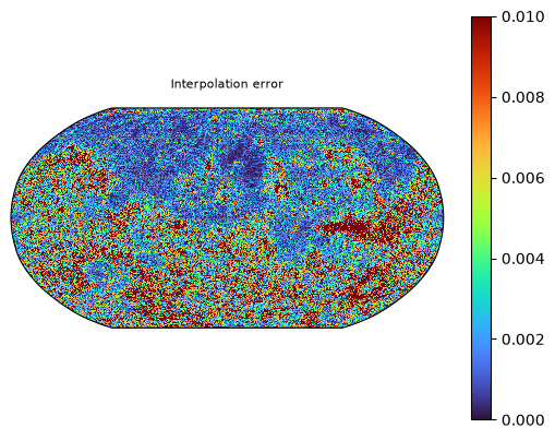
../_images/8b78e79fb56e3c4cc7f91ca3b74011aba01e68aa0a280f5bf7a5110431b4cbe8.png

The round-trip \(\mathrm{ISHT}(\mathrm{SHT}(u))\) is not exact because the equiangular grid cannot resolve all modes — the highest frequencies are lost to truncation. Let us plot the pointwise reconstruction error:

plot_sphere((isht(coeffs).cpu() - data).abs(), cmap=cmap,
            title="Interpolation error", colorbar=True, gridlines=True,
            vmin=0, vmax=0.01)

<cartopy.mpl.geocollection.GeoQuadMesh at 0x3c7d237a0>

../_images/7172e5875dbc613fff5f8e7ca1f28499336ed347f1ff47d90926a38704555562.png

Differentiability#

Since the SHT and ISHT are implemented as PyTorch modules, they support automatic differentiation out of the box. This lets us optimize spectral coefficients directly with gradient descent.

As a demonstration, we define a small SpectralModel that holds learnable spectral coefficients \(\theta \in \mathbb{C}^{l_{\max} \times m_{\max}}\) and synthesizes a grid field via the inverse SHT. We then fit these coefficients to match the Mars elevation data by minimizing the mean squared error:

class SpectralModel(nn.Module):
    def __init__(self, n_modes, out_dims):
        super().__init__()
        self.isht = InverseRealSHT(out_dims[0], out_dims[1], lmax=n_modes, mmax=n_modes, grid="equiangular").to(device)
        self.coeffs = nn.Parameter(torch.randn(self.isht.lmax, self.isht.mmax, dtype=torch.complex128))

    def forward(self):
        return self.isht(self.coeffs)

sh_model = SpectralModel(120, (nlat, nlon)).to(device)
sh_model

SpectralModel(
  (isht): InverseRealSHT(
    nlat=512, nlon=1024,
     lmax=120, mmax=120,
     grid=equiangular, csphase=True
  )
)

We optimize the coefficients using Adam. Because the ISHT is differentiable, gradients flow from the pixel-space loss all the way back to the spectral coefficients:

optimizer = torch.optim.Adam(sh_model.parameters(), lr = 5e-2)

pbar = tqdm(range(500), desc="Spectral fitting")
for iter in pbar:

    loss = (sh_model() - signal).pow(2).mean()

    optimizer.zero_grad()
    loss.backward()
    optimizer.step()

    if iter % 10 == 0:
        pbar.set_postfix_str(f"loss={loss.item():.6f}")

Spectral fitting: 100%|██████████| 500/500 [00:06<00:00, 71.86it/s, loss=0.000257] 

Let us plot the approximation:

plot_sphere(sh_model().detach().cpu(), cmap=cmap, gridlines=True)

<cartopy.mpl.geocollection.GeoQuadMesh at 0x3cb1d63f0>

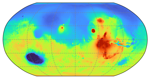
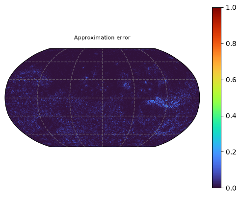
../_images/1ad60da067c080214cc74159ba0fb23350e82cd405d02f3677c26601b06f1aae.png

The model uses only 120 modes, so it cannot capture the finest details. The error map shows where the band-limited approximation deviates from the full-resolution data:

plot_sphere((sh_model().detach() - signal).abs().cpu(), cmap=cmap,
            title="Approximation error", colorbar=True, gridlines=True,
            vmin=0, vmax=1)

<cartopy.mpl.geocollection.GeoQuadMesh at 0x3d574a3f0>

../_images/f32ef5704885664bd6ee49209b8fac5bff23e2548258dac99765cc721aab9d92.png

Conclusion#

This concludes our introduction to torch-harmonics.

Getting started with torch-harmonics#