Spherical harmonic transforms

This guide explains the mathematical formulation behind the scalar and vector spherical harmonic transforms (SHT) in torch-harmonics, the available normalization conventions, and the supported quadrature grids.

1. Spherical harmonics

The spherical harmonics \(Y_l^m(\theta, \lambda)\) form a complete orthogonal basis for square-integrable functions on the sphere \(S^2\). Here \(\theta\) denotes colatitude (\(0\) at the north pole, \(\pi\) at the south pole) and \(\lambda\) denotes longitude (\(0\) to \(2\pi\)). They are separable into an associated Legendre polynomial in colatitude and a complex exponential in longitude:

\[ Y_l^m(\theta, \lambda) = P_l^m(\cos\theta)\,e^{im\lambda} \]

where \(l \ge 0\) is the degree and \(0 \le m \le l\) is the order.

1.1 Normalization conventions

The normalization of the associated Legendre polynomials \(P_l^m\) (and hence of \(Y_l^m\)) is controlled by the norm parameter. torch-harmonics supports three conventions:

norm	Convention	Inner-product property
"ortho"	Orthonormal (4\(\pi\)-normalized)	\(\langle Y_l^m, Y_{l'}^{m'}\rangle = \delta_{ll'}\delta_{mm'}\)
"schmidt"	Schmidt semi-normalized	Carries \(\sqrt{(l-m)!/(l+m)!}\) but omits \(\sqrt{2l+1}\)
"unnorm"	Unnormalized	Bare three-term recurrence; not recommended for general use

The inner product is \(\langle f, g \rangle = \int_0^{2\pi}\int_0^{\pi} f\,\bar{g}\,\sin\theta\,d\theta\,d\lambda\).

The ortho convention is the default and is standard in physics. The Schmidt convention is common in geomagnetism and gravity-field modelling. The unnorm convention is provided for special-purpose work but is not recommended because coefficient magnitudes grow with degree.

1.2 Condon–Shortley phase

The csphase parameter controls whether the Condon–Shortley phase factor \((-1)^m\) is included in the associated Legendre polynomials. When csphase=True (default), the standard physics convention is used, in which the raising/lowering operators have real, positive matrix elements. Setting csphase=False removes this factor, following the geodesy/geomagnetism convention.

2. Forward scalar SHT

Given a real-valued signal \(f(\theta, \lambda)\) sampled on the sphere, the forward scalar SHT (RealSHT) computes the spherical harmonic coefficients

\[ \hat{f}_l^m = \int_0^{2\pi} \int_0^{\pi} f(\theta, \lambda)\, \overline{Y_l^m(\theta, \lambda)}\, \sin\theta\; d\theta\; d\lambda \]

In practice the integral is evaluated in two stages:

1. Longitudinal FFT: a real FFT along the \(\lambda\) direction extracts the Fourier modes \(\tilde{f}_m(\theta_k)\) at each quadrature node \(\theta_k\).

2. Legendre quadrature: a Gauss-type quadrature contracts the Fourier modes with the associated Legendre polynomials and quadrature weights \(q_k\):

\[ \hat{f}_l^m = 2\pi \sum_{k=0}^{N_\theta - 1} \tilde{f}_m(\theta_k)\, P_l^m(\cos\theta_k)\, q_k \]

3. Inverse scalar SHT

Given complex spherical harmonic coefficients \(\hat{f}_l^m\), the inverse scalar SHT (InverseRealSHT) reconstructs the real-valued signal on the sphere:

\[ f(\theta, \lambda) = \sum_{l=0}^{l_{\max}-1} \sum_{m=0}^{m_{\max}-1} \hat{f}_l^m\, Y_l^m(\theta, \lambda) \]

The synthesis is carried out in two stages:

1. Legendre synthesis: contracts the coefficients with the associated Legendre polynomials to produce Fourier modes at each grid latitude:

\[ \tilde{f}_m(\theta_k) = \sum_{l=m}^{l_{\max}-1} \hat{f}_l^m\, P_l^m(\cos\theta_k) \]

2. Inverse FFT: an inverse real FFT along the longitudinal direction reconstructs the spatial signal \(f(\theta_k, \lambda_j)\).

Note

The inverse real FFT (C2R transform) expects the DC component (\(m = 0\)) and, when nlon is even, the Nyquist component (\(m = N_\lambda / 2\)) to be purely real. The module zeros out the imaginary parts of these components before calling the transform.

4. Quadrature grids

The accuracy of the SHT depends on the quadrature rule used for the latitudinal integration. torch-harmonics supports the following grid types:

grid	Quadrature	Poles included	Polynomial exactness
"legendre-gauss"	Gauss–Legendre	No	\(2N_{\text{lat}} - 1\)
"lobatto"	Gauss–Lobatto	Yes (both)	\(2N_{\text{lat}} - 3\)
"equiangular"	Clenshaw–Curtis	Yes (both)	\(N_{\text{lat}} - 1\) (odd), \(N_{\text{lat}}\) (even)
"equiangular-trapezoidal"	Extended trapezoidal	Yes (both)	–

The default is "equiangular", which provides uniformly spaced latitudes and is the most common choice for climate and weather applications. "legendre-gauss" achieves the highest polynomial exactness per grid point and is preferred when maximum accuracy at low resolution is needed.

5. Example: scalar SHT round-trip

import matplotlib.pyplot as plt
import torch

import torch_harmonics as th
from torch_harmonics.plotting import plot_sphere
from torch_harmonics.utils import load_mola_elevation

nlat, nlon = 128, 256
signal = load_mola_elevation(nlat, nlon).unsqueeze(0)

sht = th.RealSHT(nlat, nlon, grid="equiangular")
isht = th.InverseRealSHT(nlat, nlon, grid="equiangular")

# forward transform
coeffs = sht(signal)

# inverse transform
reconstructed = isht(coeffs)

err = (signal - reconstructed).abs().max().item()
print(f"coeffs shape: {coeffs.shape}")
print(f"Max reconstruction error: {err:.2e}")

coeffs shape: torch.Size([1, 64, 64])
Max reconstruction error: 3.40e-01

/opt/anaconda/envs/torch-harmonics/lib/python3.12/site-packages/torch_harmonics/truncation.py:168: UserWarning: Default SHT truncation changed in v0.9.0: equiangular/equiangular-trapezoidal grids now truncate to (nlat+1)//2. Specify lmax explicitly to override.
  lmax = lmax or _truncate_lmax(nlat, grid)

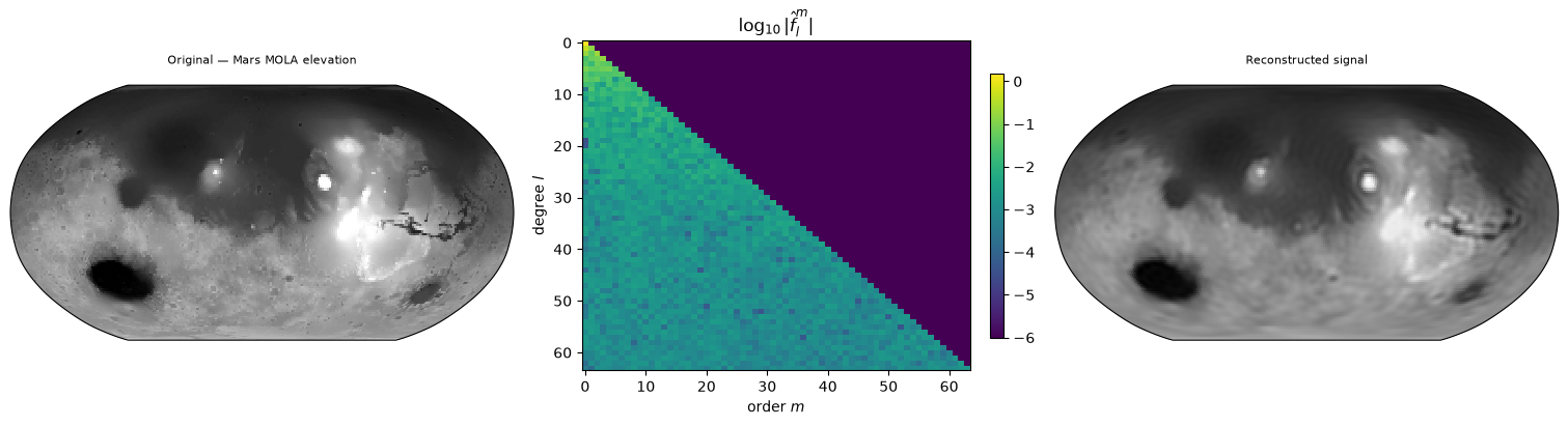
fig = plt.figure(figsize=(15, 4), layout="constrained")
subfigs = fig.subfigures(1, 3)

plot_sphere(signal[0], fig=subfigs[0], cmap="gray", title="Original — Mars MOLA elevation")

# spectral coefficients (keep as imshow)
ax = subfigs[1].add_subplot()
spec = coeffs[0].abs().log10().clamp(min=-6)
im = ax.imshow(spec, aspect="auto", cmap="viridis")
ax.set_title("$\\log_{10}|\\hat{f}_l^m|$")
ax.set_xlabel("order $m$")
ax.set_ylabel("degree $l$")
subfigs[1].colorbar(im, ax=ax, shrink=0.8)

plot_sphere(reconstructed[0], fig=subfigs[2], cmap="gray", title="Reconstructed signal")

plt.show()

6. Forward vector SHT

A tangential vector field on the sphere can be written as $\mathbf{v}(\theta,\lambda) = v_\theta,\hat{e}_\theta

• v_\lambda,\hat{e}_\lambda\(. The vector SHT ({class}`~torch_harmonics.RealVectorSHT`) decomposes this field into **spheroidal** and **toroidal** spectral coefficients \)\hat{s}_l^m\( and \)\hat{t}_l^m$:

\[ \hat{s}_l^m = \frac{1}{l(l+1)} \int_0^{2\pi} \int_0^{\pi} \left[ v_\theta\, \frac{\partial \overline{Y_l^m}}{\partial \theta} + v_\lambda\, \frac{1}{\sin\theta} \frac{\partial \overline{Y_l^m}}{\partial \lambda} \right] \sin\theta\; d\theta\; d\lambda \]

\[ \hat{t}_l^m = \frac{1}{l(l+1)} \int_0^{2\pi} \int_0^{\pi} \left[ v_\theta\, \frac{1}{\sin\theta} \frac{\partial \overline{Y_l^m}}{\partial \lambda} - v_\lambda\, \frac{\partial \overline{Y_l^m}}{\partial \theta} \right] \sin\theta\; d\theta\; d\lambda \]

As with the scalar SHT, the longitudinal integrals are evaluated with a real FFT and the latitudinal integrals via Gauss-type quadrature using the derivatives of the associated Legendre polynomials.

7. Inverse vector SHT

Given spheroidal and toroidal spectral coefficients, the inverse vector SHT (InverseRealVectorSHT) reconstructs the tangential vector field:

\[ v_\theta(\theta,\lambda) = \sum_{l=0}^{l_{\max}-1} \sum_{m=0}^{m_{\max}-1} \left[ \hat{s}_l^m\, \frac{\partial Y_l^m}{\partial \theta} + \hat{t}_l^m\, \frac{1}{\sin\theta} \frac{\partial Y_l^m}{\partial \lambda} \right] \]

\[ v_\lambda(\theta,\lambda) = \sum_{l=0}^{l_{\max}-1} \sum_{m=0}^{m_{\max}-1} \left[ \hat{s}_l^m\, \frac{1}{\sin\theta} \frac{\partial Y_l^m}{\partial \lambda} - \hat{t}_l^m\, \frac{\partial Y_l^m}{\partial \theta} \right] \]

A Legendre synthesis contracts the coefficients with the derivatives of the associated Legendre polynomials, followed by an inverse real FFT to recover the spatial components.

8. Example: vector SHT round-trip

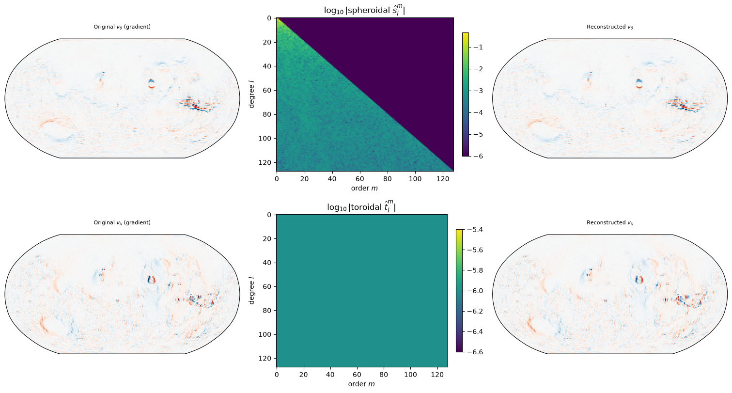
To demonstrate the vector SHT on a physically meaningful field, we compute the surface gradient of the Mars MOLA elevation map spectrally: the scalar SHT coefficients \(\hat{f}_l^m\) are placed into the spheroidal channel (with the toroidal channel set to zero), and the inverse vector SHT synthesises \(\nabla_H f\). We then verify that a forward–inverse round-trip recovers the same vector field.

We switch to the legendre-gauss grid here, which avoids the coordinate singularity at the poles (\(\sin\theta = 0\)) and provides higher quadrature exactness (\(2N_{\text{lat}} - 1\)).

# use legendre-gauss to avoid pole singularity
nlat_v, nlon_v = 128, 256
grid_v = "legendre-gauss"

# resample the Mars elevation onto the legendre-gauss grid via SHT
sht_eq = th.RealSHT(nlat, nlon, lmax=nlat_v, mmax=nlon_v // 2 + 1, grid="equiangular")
isht_lg = th.InverseRealSHT(nlat_v, nlon_v, lmax=nlat_v, mmax=nlon_v // 2 + 1, grid=grid_v)
signal_lg = isht_lg(sht_eq(signal))

# scalar SHT on the legendre-gauss grid
sht_v = th.RealSHT(nlat_v, nlon_v, grid=grid_v)
scalar_coeffs = sht_v(signal_lg)

# build gradient vector field: spheroidal = scalar coefficients, toroidal = 0
grad_coeffs = torch.zeros(1, 2, *scalar_coeffs.shape[1:], dtype=scalar_coeffs.dtype)
grad_coeffs[:, 0] = scalar_coeffs

# synthesise the gradient vector field
ivsht = th.InverseRealVectorSHT(nlat_v, nlon_v, grid=grid_v)
vector_field = ivsht(grad_coeffs)

# round-trip: forward vector SHT then inverse
vsht = th.RealVectorSHT(nlat_v, nlon_v, grid=grid_v)
coeffs = vsht(vector_field)
reconstructed = ivsht(coeffs)

err = (vector_field - reconstructed).abs().max().item()
print(f"vector field shape: {vector_field.shape}")
print(f"coeffs shape:       {coeffs.shape}")
print(f"Max reconstruction error: {err:.2e}")

vector field shape: torch.Size([1, 2, 128, 256])
coeffs shape:       torch.Size([1, 2, 128, 128])
Max reconstruction error: 1.91e-06

fig = plt.figure(figsize=(15, 8), layout="constrained")
subfigs = fig.subfigures(2, 3)

for i, (comp, label) in enumerate([(r"$v_\theta$", "spheroidal $\\hat{s}_l^m$"),
                                    (r"$v_\lambda$", "toroidal $\\hat{t}_l^m$")]):
    vmax = vector_field[0, i].abs().max().item()

    plot_sphere(vector_field[0, i], fig=subfigs[i, 0], cmap="RdBu",
                title=f"Original {comp} (gradient)", vmin=-vmax, vmax=vmax)

    # spectral coefficients (keep as imshow)
    ax = subfigs[i, 1].add_subplot()
    spec = coeffs[0, i].abs().log10().clamp(min=-6)
    im = ax.imshow(spec, aspect="auto", cmap="viridis")
    ax.set_title(f"$\\log_{{10}}|${label}$|$")
    ax.set_xlabel("order $m$")
    ax.set_ylabel("degree $l$")
    subfigs[i, 1].colorbar(im, ax=ax, shrink=0.8)

    plot_sphere(reconstructed[0, i], fig=subfigs[i, 2], cmap="RdBu",
                title=f"Reconstructed {comp}", vmin=-vmax, vmax=vmax)

plt.show()

9. cuFFT precision note

All SHT modules use cuFFT (via torch.fft.rfft / torch.fft.irfft) for the longitudinal Fourier transform. When running in float16 or bfloat16 precision, cuFFT requires the transformed dimension (nlon) to be a power of two. If your grid does not satisfy this constraint and the module is called inside a torch.autocast context, guard it with an inner context that disables autocast:

with torch.autocast(device_type="cuda", dtype=torch.float16):
    # ... other half-precision work ...
    with torch.autocast(device_type="cuda", enabled=False):
        coeffs = sht(signal.float())

Summary

• The scalar SHT decomposes a function on the sphere into spherical harmonic coefficients \(\hat{f}_l^m\) via FFT + Legendre quadrature. The inverse SHT reconstructs the signal from its coefficients.

• The vector SHT decomposes a tangential vector field into spheroidal and toroidal spectral coefficients using derivatives of the associated Legendre polynomials.

• Three normalization conventions (ortho, schmidt, unnorm) and optional Condon–Shortley phase are supported.

• Four quadrature grids are available, trading off accuracy and grid structure.

For the full parameter documentation, see RealSHT, InverseRealSHT, RealVectorSHT, and InverseRealVectorSHT.