
Differentiable shallow water equations#
This notebook solves the rotating shallow water equations (SWE) on the sphere
using the spectral methods provided by torch-harmonics. The SWE describe
the evolution of a thin fluid layer under gravity and rotation:
where \(\mathbf{u}\) is the horizontal velocity, \(\zeta = \nabla \times \mathbf{u}\) the relative vorticity, \(f\) the Coriolis parameter, and \(\Phi = g h\) the geopotential.
The solver works in spectral space (vorticity–divergence formulation) and uses third-order Adams–Bashforth time integration. Because the SHT and all operations are implemented as differentiable PyTorch modules, gradients can be propagated through the entire time integration.
Setup#
import torch
import matplotlib.pyplot as plt
import matplotlib.animation as animation

from math import ceil, floor
from tqdm.auto import tqdm

from torch_harmonics.examples import ShallowWaterSolver
/opt/anaconda/envs/torch-harmonics/lib/python3.12/site-packages/tqdm/auto.py:21: TqdmWarning: IProgress not found. Please update jupyter and ipywidgets. See https://ipywidgets.readthedocs.io/en/stable/user_install.html
  from .autonotebook import tqdm as notebook_tqdm
device = torch.device('cuda' if torch.cuda.is_available() else 'cpu')
Solver configuration#
We set up a ShallowWaterSolver on a 512 × 1024 grid with spectral
truncation at \(l_{\max} = 128\). The time step is 75 s and we integrate
for 12 simulated days (≈ 288 hours):
# initialize parameters:
nlat = 512
nlon = 2*nlat
lmax = ceil(128)
mmax = lmax
# timestepping
dt = 75
maxiter = 12*int(86400/dt)

# initialize solver class
swe_solver = ShallowWaterSolver(nlat, nlon, dt, lmax=lmax, mmax=mmax).to(device)

lons = swe_solver.lons
lats = swe_solver.lats

jj, ii = torch.triu_indices(lmax, mmax)
Initial condition — Galewsky jet#
The Galewsky test case initialises a barotropically unstable zonal jet with a localised perturbation in the height field. The jet breaks up into a train of vortices over several days, providing a stringent test of the solver’s accuracy and stability:
uspec0 = swe_solver.galewsky_initial_condition()
/opt/anaconda/envs/torch-harmonics/lib/python3.12/site-packages/torch/functional.py:504: UserWarning: torch.meshgrid: in an upcoming release, it will be required to pass the indexing argument. (Triggered internally at /Users/runner/work/pytorch/pytorch/aten/src/ATen/native/TensorShape.cpp:4217.)
  return _VF.meshgrid(tensors, **kwargs)  # type: ignore[attr-defined]
Time integration#
We integrate using third-order Adams–Bashforth. The first two steps fall back to lower-order schemes (forward Euler, then second-order AB) to bootstrap the multistep method. Hyperdiffusion is applied implicitly to the vorticity and divergence fields to control grid-scale noise:
dudtspec = torch.zeros(3, 3, swe_solver.lmax, swe_solver.mmax, dtype=torch.complex128, device=device)
inew = 0
inow = 1
iold = 2

uspec = uspec0.clone().to(device)

# save for later:
nskip = 50
utspec = torch.zeros(floor(maxiter//nskip) + 1, *uspec.shape).cdouble().to(device)

pbar = tqdm(range(maxiter+1), desc="SWE integration")
with torch.inference_mode():
    for iter in pbar:
        t = iter*dt

        if iter % nskip == 0:
            utspec[iter//nskip] = uspec
            pbar.set_postfix_str(f"t={t/3600:.2f}h")

        dudtspec[inew] = swe_solver.dudtspec(uspec)

        # update vort,div,phiv with third-order adams-bashforth.
        # forward euler, then 2nd-order adams-bashforth time steps to start.
        if iter == 0:
            dudtspec[inow] = dudtspec[inew]
            dudtspec[iold] = dudtspec[inew]
        elif iter == 1:
            dudtspec[iold] = dudtspec[inew]

        uspec = uspec + swe_solver.dt*( (23./12.) * dudtspec[inew] - (16./12.) * dudtspec[inow] + (5./12.) * dudtspec[iold] )

        # implicit hyperdiffusion for vort and div.
        uspec[1:] = swe_solver.hyperdiff * uspec[1:]
        # cycle through the indices
        inew = (inew - 1) % 3
        inow = (inow - 1) % 3
        iold = (iold - 1) % 3
SWE integration: 100%|██████████| 13825/13825 [14:57<00:00, 15.40it/s, t=287.50h]
Snapshot#
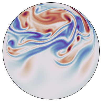
Let us visualise the vorticity field at the end of the integration:
fig = plt.figure()
im = swe_solver.plot_specdata(uspec[1], fig, cmap="twilight_shifted")
plt.show()
Animation#
We render the full time series of the vorticity field as an animated GIF.
Set plot_pvrt = True to visualise potential vorticity instead:
import os
os.makedirs("plots", exist_ok=True)

# prepare figure for animation
fig = plt.figure(figsize=(8, 6), dpi=72)
moviewriter = animation.writers['pillow'](fps=20)
moviewriter.setup(fig, './plots/zonal_jet.gif', dpi=72)

plot_pvrt = False

for i in tqdm(range(utspec.shape[0]), desc="Rendering frames"):
    t = i*nskip*dt

    if plot_pvrt:
        variable = swe_solver.potential_vorticity(utspec[i])
    else:
        variable = swe_solver.spec2grid(utspec[i, 1])

    plt.clf()
    swe_solver.plot_griddata(variable, fig, cmap="twilight_shifted", antialiased=False)
    plt.draw()
    moviewriter.grab_frame()

moviewriter.finish()
Rendering frames: 100%|██████████| 277/277 [01:21<00:00, 3.42it/s]
Conservation of potential vorticity#
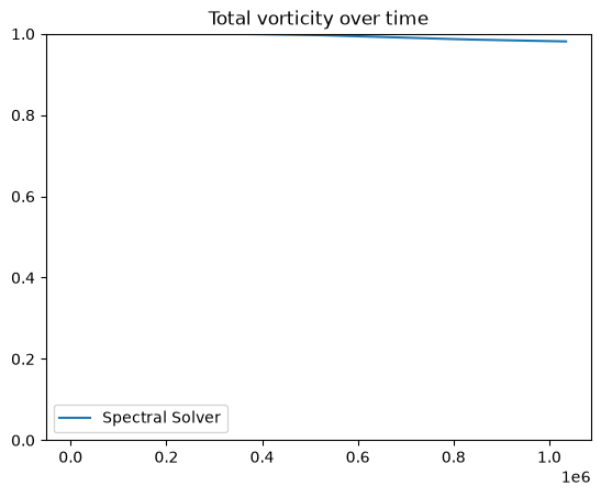
The potential vorticity \(q = (\zeta + f) / \Phi\) is a materially conserved quantity — it should remain constant following fluid parcels. We verify this by computing the total spectral energy of \(q\) at each saved time step and checking that it stays close to its initial value:
pvrttspec = torch.zeros(floor(maxiter//nskip) + 1, lmax, mmax).cdouble().to(device)
for i in range(utspec.shape[0]):
    pvrttspec[i] = swe_solver.grid2spec(swe_solver.potential_vorticity(utspec[i]))
total_vrt = pvrttspec.abs()**2
# total_vrt = utspec[..., 1, :, :].abs()**2
total_vrt = torch.sqrt(torch.sum(total_vrt[..., :1], dim=(-1, -2)) + torch.sum(2 * total_vrt[..., 1:], dim=(-1, -2))).cpu()
t = nskip*dt * torch.arange(utspec.shape[0])

plt.plot(t, total_vrt / total_vrt[0], label='Spectral Solver')
plt.title('Total vorticity over time')
plt.ylim((0,1))
plt.legend(loc='lower left')
<matplotlib.legend.Legend at 0x157fd2930>