Conditioning of the SHT

This notebook investigates the conditioning of the spherical harmonic transform (SHT) by constructing the Vandermonde matrix \(S\) and analyzing its Gramian \(G = S^T \mathrm{diag}(\omega)\, S\).

A well-conditioned SHT means that the analysis (forward) and synthesis (inverse) steps are numerically stable. We verify this by checking that the condition number of the Gramian is close to 1 and that the round-trip \(\mathrm{ISHT}(\mathrm{SHT}(u)) \approx u\) reproduces the input.

Setup

import numpy as np
import torch

from torch_harmonics.quadrature import legendre_gauss_weights, clenshaw_curtiss_weights
from torch_harmonics import RealSHT, InverseRealSHT

import matplotlib.pyplot as plt

from torch_harmonics.plotting import plot_sphere

nlat = 32
nlon = 2*nlat
grid = "legendre-gauss"

# for quadrature and plotting
if grid == "legendre-gauss":
    lmax = mmax = nlat
    xq, wq = legendre_gauss_weights(nlat)
elif grid =="equiangular":
    lmax = mmax = nlat//2-1
    xq, wq = clenshaw_curtiss_weights(nlat)

sht = RealSHT(nlat, nlon, lmax=lmax, mmax=mmax, grid=grid)
isht = InverseRealSHT(nlat, nlon, lmax=lmax, mmax=mmax, grid=grid)

lat = torch.arccos(xq)
omega = torch.pi * wq.float() / nlat
omega = omega.reshape(-1, 1).repeat(1, nlon)

omega.sum()

tensor(12.5664)

Constructing the Vandermonde matrix

The Vandermonde matrix \(S\) encodes the action of the inverse SHT: \(u = S\,\theta\), where \(\theta\) are the spectral coefficients and \(u\) the grid values. We construct it column by column, applying the ISHT to each unit basis vector \(e_{l,m}\) in spectral space.

# forming the Vandermonde matrix
nmodes = int(lmax * (lmax+1) / 2)
e = torch.zeros(nmodes, lmax, mmax, dtype=torch.complex64)

midx = lambda l,m : l*(l+1)//2 + m

for l in range(lmax):
    for m in range(l+1):
        e[midx(l,m), l, m] = 1.0

vdm = isht(e) # nmodes x nlat x nlon

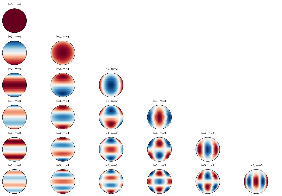
Each column of the Vandermonde matrix corresponds to a spherical harmonic \(Y_l^m\). Let us visualize the first few to verify the construction:

plt_lmax = 6

fig = plt.figure(figsize=(12, 8), layout='constrained')
subfigs = fig.subfigures(plt_lmax, plt_lmax)

for l in range(plt_lmax):
    for m in range(l+1):
        plot_sphere(vdm[midx(l,m)], fig=subfigs[l, m], projection="orthographic", title=f"l={l}, m={m}", lat=(lat - np.pi/2))

Gramian analysis

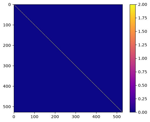
The Gramian \(G = S^T \mathrm{diag}(\omega)\, S\) captures how well the quadrature weights preserve orthogonality of the spherical harmonics. For an exact quadrature rule, \(G\) is the identity matrix (up to a scaling factor). Any deviation indicates numerical error in the transform.

gramian = torch.einsum("iqr,jqr,qr->ij", vdm, vdm, omega)

plt.imshow(gramian, interpolation="nearest", cmap="plasma")
plt.colorbar()

<matplotlib.colorbar.Colorbar at 0x16b444050>

print(torch.max(gramian))
print(torch.argmax(gramian))
print(torch.min(gramian))
print(torch.argmin(gramian))

tensor(2.0000)
tensor(113206)
tensor(-2.2352e-07)
tensor(178452)

The condition number of \(G\) tells us how much numerical error is amplified through the analysis–synthesis cycle. A condition number close to 1 indicates a well-conditioned transform:

np.linalg.cond(gramian)

np.float32(2.000001)

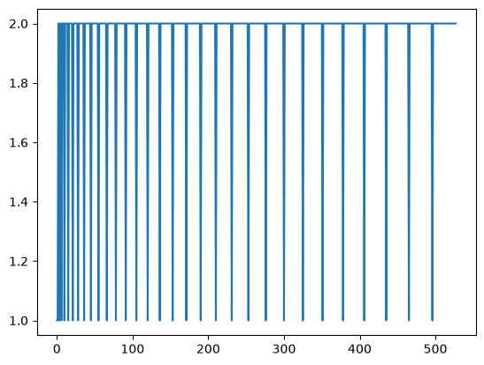
The diagonal entries of \(G\) correspond to the norms \(\|Y_l^m\|^2\) under the discrete quadrature. A flat diagonal confirms that all modes are weighted equally:

plt.plot(np.diag(gramian))

[<matplotlib.lines.Line2D at 0x16b4fddc0>]

Projection operator \(S^{-1} S\)

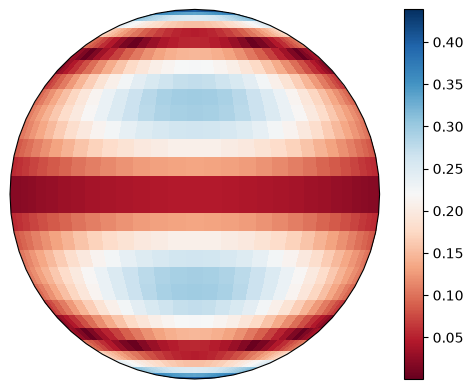
We can also construct the full forward (\(S\)) and inverse (\(S^{-1}\)) matrices explicitly and examine their product. The composition \(S^{-1} S\) acts as a projection operator from grid space onto the space of band-limited functions. For a point that lies in the column space of \(S^{-1}\), the round-trip is exact.

# forming the Vandermonde matrix
nmodes = int(lmax * (lmax+1) / 2)

e = torch.zeros(lmax, mmax, lmax, mmax, dtype=torch.complex64)
for l in range(lmax):
    for m in range(l+1):
        e[l, m, l, m] = 1.0

Sinv = isht(e).cfloat() # l x m x nlat x nlon

e = torch.zeros(nlat, nlon, nlat, nlon, dtype=torch.float32)
for lat in range(nlat):
    for lon in range(nlon):
        e[lat, lon, lat, lon] = 1.0

S = sht(e) # nlat x nlon x l x m

out = torch.einsum("lmop,lmqr->lopqr", Sinv, Sinv.conj())

plot_sphere(out[3, 29, 16].abs(), projection="orthographic", colorbar=True)

<cartopy.mpl.geocollection.GeoQuadMesh at 0x16b667d10>

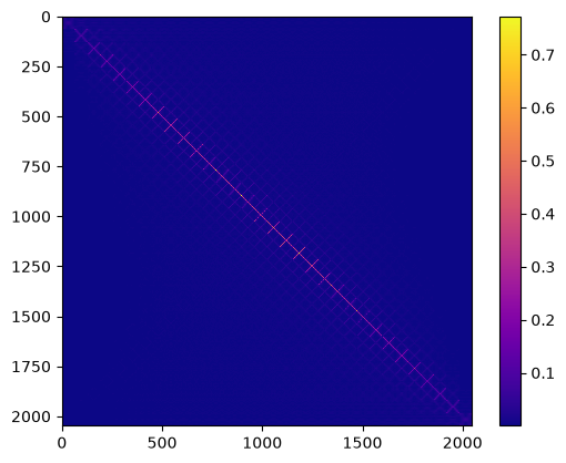
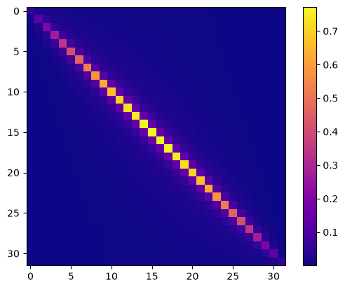
The product \(S^{-1} S\) should approximate an identity matrix. Let us visualize it as a dense matrix and inspect individual slices:

SS = torch.einsum("lmqr, oplm->qrop", Sinv, S)

plt.imshow(SS.reshape(nlat*nlon, nlat*nlon).abs(), interpolation="nearest", cmap="plasma")
plt.colorbar()

<matplotlib.colorbar.Colorbar at 0x16b6fa8d0>

plt.imshow(SS[:,0,:,0].abs(), interpolation="nearest", cmap="plasma")
plt.colorbar()

<matplotlib.colorbar.Colorbar at 0x16b7c50a0>

Round-trip test

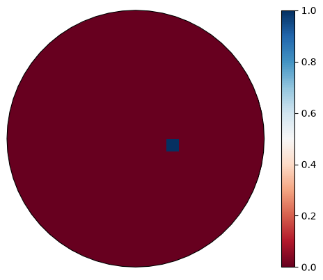
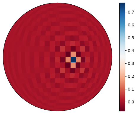
As a final sanity check, we apply the SHT round-trip to a point source (delta function on the grid). A well-conditioned transform will spread the point source into a smooth band-limited interpolant, then reconstruct it faithfully:

field = torch.zeros(nlat, nlon)
field[16,3] = 1.0

plot_sphere(field, projection="orthographic", colorbar=True)
plot_sphere(isht(sht(field)), projection="orthographic", colorbar=True)

<cartopy.mpl.geocollection.GeoQuadMesh at 0x16e204ec0>