Attention on the sphere

This guide explains the two spherical attention layers in torch-harmonics: global AttentionS2 and local NeighborhoodAttentionS2. Both adapt standard scaled dot-product attention to the sphere by incorporating the numerical quadrature weights of the grid into the attention mechanism, following Bonev et al., NeurIPS 2025.

1. From planar to spherical attention

Standard scaled dot-product attention computes, for every query position \(x'\), a weighted sum of values over a set of key positions:

\[ \text{Attn}(Q, K, V)_{x'} = \sum_{x} \text{softmax}_{x}\!\left( \frac{Q(x') \cdot K(x)}{\sqrt{d_k}} \right)\, V(x) \]

On a flat, uniformly-spaced grid every point carries equal weight, so the softmax normalisation alone is sufficient. On the sphere, however, grid points near the poles are over-represented relative to their solid angle: an equiangular grid has far more points per unit area near the poles than at the equator.

To make attention geometrically faithful, we need to turn the sum into a quadrature approximation of a continuous integral over the sphere.

2. Quadrature-weighted attention

The key insight is to fold the spherical quadrature weights \(q_i\) into the softmax. Instead of normalising by the raw exponentials, we normalise by a weighted sum:

\[ \text{Attn}(Q, K, V)_{x'} = \frac{ \sum_{x} q(x)\, \exp\!\left(\frac{Q(x') \cdot K(x)}{\sqrt{d_k}}\right)\, V(x) }{ \sum_{x} q(x)\, \exp\!\left(\frac{Q(x') \cdot K(x)}{\sqrt{d_k}}\right) } \]

where \(q(x) = 2\pi\, w_k / N_\lambda\) is the spherical quadrature weight at input point \(x = (\theta_k, \lambda_j)\).

Implementation via log-weights

Because the exponential is inside both numerator and denominator, we can equivalently add \(\log q(x)\) to the pre-softmax attention scores:

\[ \alpha_{x',x} = \text{softmax}_{x}\!\left( \frac{Q(x') \cdot K(x)}{\sqrt{d_k}} + \log q(x) \right) \]

This is passed directly as the attn_mask argument to PyTorch’s scaled_dot_product_attention, making it a drop-in replacement for standard attention with minimal code changes.

Why this matters

Incorporating the quadrature weights makes the attention layer:

• Resolution-agnostic: the same learned weights can be evaluated on different grid resolutions (though the learned features remain resolution dependent).

• Approximately \(SO(3)\)-equivariant: the underlying integral is invariant under rotations (the Haar measure on \(S^2\)), so the discretised version inherits approximate equivariance.

3. Global attention (AttentionS2)

Global attention lets every output point attend to all input points. The cost is \(\mathcal{O}(N^2)\) in the number of grid points. The forward pass follows the standard multi-head attention pattern:

1. Linear projections: project the input into queries \(Q\), keys \(K\), and values \(V\) using pointwise (1×1) convolutions.

2. Reshape into num_heads independent attention heads.

3. Scaled dot-product attention with the log-quadrature-weight mask.

4. Output projection: another pointwise convolution.

The module supports self-attention (default) and cross-attention (pass separate key/value tensors).

4. Neighborhood attention (NeighborhoodAttentionS2)

For high-resolution grids, global attention becomes prohibitively expensive. Neighborhood attention restricts each output point to attend only to the input points inside a geodesic disk of radius theta_cutoff:

\[ D(x') = \{x \in S^2 : d(x, x') \le \theta_\text{cutoff}\} \]

where \(d(\cdot, \cdot)\) is the great-circle distance. This reduces the cost from \(\mathcal{O}(N^2)\) to \(\mathcal{O}(kN)\), where \(k\) is the number of neighbors.

Shared structure with DISCO convolutions

The sparse neighborhood structure is precomputed using the same discrete-continuous construction as the DISCO convolutions (see DISCO convolutions on the sphere). Specifically, the support (index information) of a zeroth-order DISCO kernel defines the indicator function of the cutoff disk. This means:

• Sparsity: only input points inside the angular cap contribute.

• Longitude invariance (p-shift): the neighborhood structure is independent of the output longitude, just like the \(\Psi\) tensor.

The relative weight of each input point depends on both its contribution to the softmax and its quadrature weight.

Online softmax

The forward pass uses a single-pass online softmax algorithm: for each output location, the neighbor list is iterated once while maintaining a running maximum and accumulator. This avoids materialising the full attention matrix and is numerically stable.

5. Example: creating attention layers

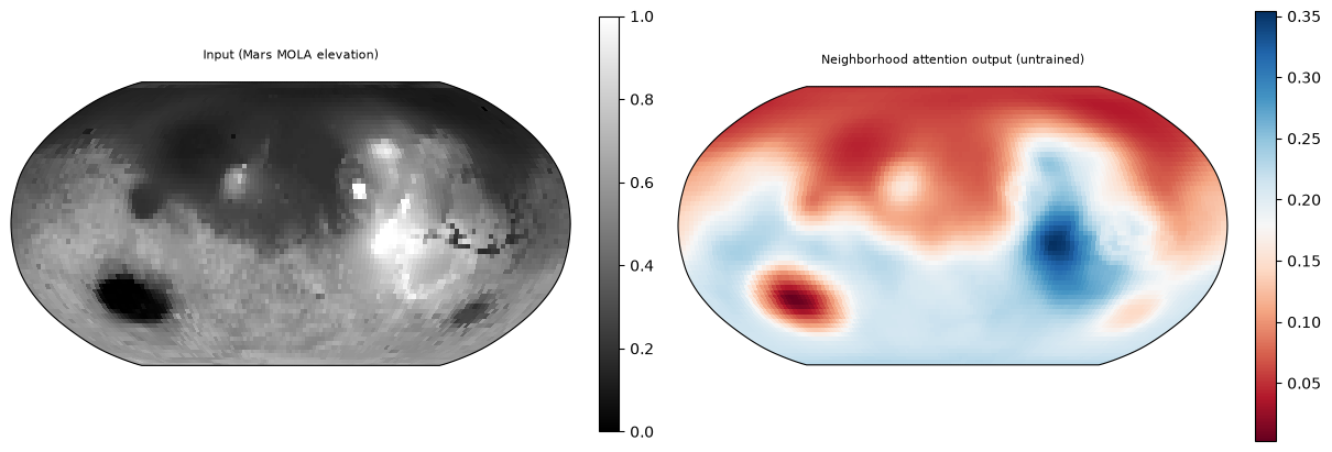
Attention layers are data-dependent — unlike convolutions, their output depends on the learned Q/K/V projections and how the input signal interacts with them through the softmax. With untrained (random) weights, the attention scores are essentially uniform, so the output carries little spatial structure. Meaningful outputs require training on a downstream task.

Here we show how to instantiate both modules and verify their input/output shapes using the Mars MOLA elevation map.

import math

import matplotlib.pyplot as plt
import torch
import torch.nn.functional as F

import torch_harmonics as th
from torch_harmonics.plotting import plot_sphere
from torch_harmonics.utils import load_mola_elevation

nlat, nlon = 64, 128
signal = load_mola_elevation(nlat, nlon).unsqueeze(0).unsqueeze(0)

in_channels = 1

# replicate to get multi-channel input
x = signal.expand(-1, in_channels, -1, -1).clone()

attn_global = th.AttentionS2(
    in_channels=in_channels,
    num_heads=1,
    in_shape=(nlat, nlon),
    out_shape=(nlat, nlon),
)

with torch.no_grad():
    y_global = attn_global(x)

print(f"Input shape:  {x.shape}")
print(f"Output shape: {y_global.shape}")

Input shape:  torch.Size([1, 1, 64, 128])
Output shape: torch.Size([1, 1, 64, 128])

6. Example: neighborhood attention

Neighborhood attention uses the same API but confines each output point to attend only within a geodesic disk of radius theta_cutoff. Even with untrained weights, the locality constraint means different output locations see different subsets of the input, producing some spatial variation.

torch.manual_seed(333)

attn_local = th.NeighborhoodAttentionS2(
    in_channels=in_channels,
    num_heads=1,
    in_shape=(nlat, nlon),
    out_shape=(nlat, nlon),
    theta_cutoff=0.2,
)

with torch.no_grad():
    y_local = attn_local(x)

print(f"Input shape:  {x.shape}")
print(f"Output shape: {y_local.shape}")

Input shape:  torch.Size([1, 1, 64, 128])
Output shape: torch.Size([1, 1, 64, 128])

fig = plt.figure(figsize=(12, 4), layout="constrained")
subfigs = fig.subfigures(1, 2)

plot_sphere(x[0, 0], fig=subfigs[0], cmap="gray",
            title="Input (Mars MOLA elevation)", colorbar=True)

plot_sphere(y_local[0, 0].detach(), fig=subfigs[1], cmap="RdBu",
            title="Neighborhood attention output (untrained)", colorbar=True)

plt.show()

7. Neighborhood sparsity

Like the DISCO convolution’s \(\Psi\) tensor, the neighborhood attention’s sparse index structure scales linearly with the number of grid points. Let’s inspect how theta_cutoff affects the number of neighbors.

for tc in [0.05, 0.1, 0.2, 0.4]:

    torch.manual_seed(333)

    attn_tc = th.NeighborhoodAttentionS2(
        in_channels=1,
        num_heads=1,
        in_shape=(nlat, nlon),
        out_shape=(nlat, nlon),
        theta_cutoff=tc,
    )
    nnz = attn_tc.psi_col_idx.numel()
    avg_neighbors = nnz / (nlat * nlon)
    print(f"theta_cutoff={tc:.2f} rad ({math.degrees(tc):5.1f} deg): "
          f"{nnz:>8,} neighbor pairs, "
          f"avg {avg_neighbors:.1f} neighbors/output")

theta_cutoff=0.05 rad (  2.9 deg):    1,272 neighbor pairs, avg 0.2 neighbors/output
theta_cutoff=0.10 rad (  5.7 deg):    3,290 neighbor pairs, avg 0.4 neighbors/output
theta_cutoff=0.20 rad ( 11.5 deg):    9,902 neighbor pairs, avg 1.2 neighbors/output
theta_cutoff=0.40 rad ( 22.9 deg):   31,154 neighbor pairs, avg 3.8 neighbors/output

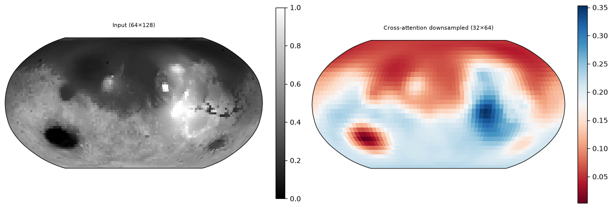
8. Cross-attention and downsampling

Both attention modules support cross-attention: pass separate key and value tensors sampled on the input grid, while the query lives on the output grid. When the input and output grids differ in resolution, this naturally performs downsampling (or upsampling for neighborhood attention).

nlat_out, nlon_out = 32, 64

torch.manual_seed(333)

attn_down = th.NeighborhoodAttentionS2(
    in_channels=in_channels,
    num_heads=1,
    in_shape=(nlat, nlon),
    out_shape=(nlat_out, nlon_out),
    theta_cutoff=0.2,
)

# query on the coarser grid, key/value on the finer grid
query = F.interpolate(signal, size=(nlat_out, nlon_out), mode="bilinear",
                      align_corners=False).expand(-1, in_channels, -1, -1).clone()
key_val = x

with torch.no_grad():
    y_down = attn_down(query, key=key_val, value=key_val)

print(f"Query shape:  {query.shape}")
print(f"Key shape:    {key_val.shape}")
print(f"Output shape: {y_down.shape}")

Query shape:  torch.Size([1, 1, 32, 64])
Key shape:    torch.Size([1, 1, 64, 128])
Output shape: torch.Size([1, 1, 32, 64])

fig = plt.figure(figsize=(12, 4), layout="constrained")
subfigs = fig.subfigures(1, 2)

plot_sphere(x[0, 0], fig=subfigs[0], cmap="gray",
            title=f"Input ({nlat}×{nlon})", colorbar=True)

plot_sphere(y_down[0, 0].detach(), fig=subfigs[1], cmap="RdBu",
            title=f"Cross-attention downsampled ({nlat_out}×{nlon_out})", colorbar=True)

plt.show()

9. Choosing theta_cutoff

theta_cutoff plays the same role as in DISCO convolutions — it controls the receptive field of each output point:

• Smaller theta_cutoff means fewer neighbors (faster, less memory) but a more local receptive field.

• Larger theta_cutoff approaches global attention in the limit (\(\theta_\text{cutoff} = \pi\) recovers full attention over the sphere).

• If not specified, it defaults to one latitudinal grid spacing: \(\pi / (N_\text{lat} - 1)\).

In practice, stacking multiple neighborhood attention layers (potentially with different resolutions in a U-Net) gives a large effective receptive field while keeping each individual layer cheap.

10. Global vs. neighborhood attention

	Global (AttentionS2)	Neighborhood (NeighborhoodAttentionS2)
Receptive field	Full sphere	Geodesic disk of radius theta_cutoff
Cost	\(\mathcal{O}(N^2)\)	\(\mathcal{O}(kN)\)
Quadrature weights	Log-weights as attn_mask	Weights folded into sparse softmax
Implementation	PyTorch scaled_dot_product_attention	Custom online-softmax kernel
Cross-attention	Yes	Yes
Up/downsampling	Downsample only	Both (via p-shift direction)
Custom CUDA kernel	No (uses PyTorch SDPA)	Yes (optional, with C++ fallback)

Summary

• Spherical attention adapts standard scaled dot-product attention to the sphere by incorporating quadrature weights into the softmax normalisation, making it a discretised integral over the sphere.

• Global attention (AttentionS2) uses all grid points as keys and achieves this via log-quadrature-weight masks.

• Neighborhood attention (NeighborhoodAttentionS2) restricts attention to a geodesic disk of radius theta_cutoff, reducing cost from \(\mathcal{O}(N^2)\) to \(\mathcal{O}(kN)\).

• The neighborhood structure reuses the DISCO sparsity pattern (compact support + p-shift), making it efficient and longitude-invariant.

• Both layers are approximately \(SO(3)\)-equivariant and resolution-agnostic.

Tip

When running on CPU, the neighborhood attention kernels are parallelised with OpenMP. Setting OMP_NUM_THREADS to the number of physical cores can significantly improve performance. The optimal thread binding depends on your hardware:

• OMP_PROC_BIND=close packs threads onto adjacent cores, which is usually best on single-socket machines where threads benefit from shared cache.

• OMP_PROC_BIND=spread distributes threads across sockets or chiplets, which can be better on multi-socket or AMD EPYC systems where aggregate memory bandwidth is the bottleneck.

For Intel OpenMP, the equivalent settings are KMP_AFFINITY=compact and KMP_AFFINITY=scatter.

export OMP_NUM_THREADS=8
export OMP_PROC_BIND=close   # or spread on multi-socket systems

For the full parameter documentation, see AttentionS2 and NeighborhoodAttentionS2.