ADAPT-VQE algorithm
This tutorial explains the implementation of Adaptive Derivative-Assembled Pseudo-Trotter VQE (ADAPT-VQE) algorithm introduced in this paper.
In VQE (see this tutorial), a parameterized wave-function using UCCSD ansatz is generated and variationally tuned to minimize the expectation value of the molecular electronic Hamiltonian. In VQE approach, we include all possible single and double excitations of electrons from the occupied spin molecular orbitals of a reference state (Hartree Fock) to the unoccupied spin molecular orbitals. The excessive depth of these quantum circuits make them ill-suited for applications in the NISQ regime.
The VQE issue has led to the ADAPT-VQE proposal in which the ansatz wave-functions is constructed through the action of a selective subset of possible unitary operators , i.e., only those operators whose inclusion in the ansatz can potentially lead to the largest decrease in the expectation value of the molecular electronic Hamiltonian. In ADAPT-VQE, the ansatz is grown iteratively by appending a sequence of unitary operators to the reference Hartree-Fock state. At each iteration, the unitary operator to be applied is chosen according to a simple criterion based on the gradient of the expectation value of the Hamiltonian. Therefore, allowing us to build a compact quantum circuit which can lead to more efficient use of quantum resources.
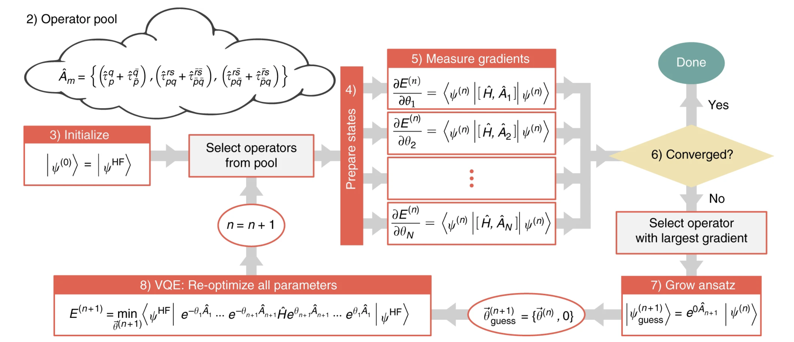
The ADAPT-VQE algorithm consists of 8 steps:
1- On classical hardware, compute one- and two-electron integrals, and transform the fermionic Hamiltonian into a qubit representation using an appropriate transformation: Jordan–Wigner, Bravyi–Kitaev, etc. For this tutorial, we will use Jordan Wigner.
2- Define an “Operator Pool”. This is simply a collection of operator definitions which will be used to construct the ansatz. For this tutorial, we will use UCCSD.
3- Initialize qubits to an appropriate reference state. Here, we use HF state to initialize the qubits.
4- Prepare a trial state with the current ansatz.
5- Measure the commutator of the Hamiltonian with each operator in the pool to get the gradient.
6- If the norm of the gradient vector is smaller than some threshold, ε, exit. otherwise, identify the operator with the largest gradient and add this single operator to the left end of the ansatz, with a new variational parameter.
7- Perform a VQE experiment to re-optimize all parameters in the ansatz.
8- go to step 4
Below is a Schematic depiction of the ADAPT-VQE algorithm
[1]:
# Requires pyscf to be installed
%pip install pyscf
Defaulting to user installation because normal site-packages is not writeable
Requirement already satisfied: pyscf in /home/cudaq/.local/lib/python3.10/site-packages (2.8.0)
Requirement already satisfied: scipy>=1.6.0 in /usr/local/lib/python3.10/dist-packages (from pyscf) (1.12.0)
Requirement already satisfied: h5py>=2.7 in /home/cudaq/.local/lib/python3.10/site-packages (from pyscf) (3.13.0)
Requirement already satisfied: setuptools in /usr/lib/python3/dist-packages (from pyscf) (59.6.0)
Requirement already satisfied: numpy!=1.16,!=1.17,>=1.13 in /usr/local/lib/python3.10/dist-packages (from pyscf) (1.26.4)
Note: you may need to restart the kernel to use updated packages.
[9]:
import cudaq

# When use mpi
#cudaq.mpi.initialize()
#print(f"My rank {cudaq.mpi.rank()} of {cudaq.mpi.num_ranks()}", flush=True)

# Set the target
# Double precision is recommended for the best performance.
if cudaq.num_available_gpus() > 0 and cudaq.has_target("nvidia"):
    cudaq.set_target("nvidia", option = "fp64")
else:
    print("CUDA or GPU support is unavailable. Running with CPU simulator. Performance may be significantly reduced.")
    cudaq.set_target("qpp-cpu")
Classical pre-processing
Here, we compute one and two-electron intgrals using Hartree Fock molecular orbitals.
[10]:
import numpy as np
from qchem.classical_pyscf import get_mol_hamiltonian

# Run HF, ccsd and compute the spin molecular hamiltonian using the HF molecular orbitals.
geometry = 'H 0.0 0.0 0.0; H 0.0 0.0 0.7474'
molecular_data = get_mol_hamiltonian(xyz= geometry, spin=0, charge=0, basis='sto3g', ccsd=True, verbose=True)

obi = molecular_data[0]
tbi = molecular_data[1]
e_nn = molecular_data[2]
nelectrons = molecular_data[3]
norbitals = molecular_data[4]
fermionic_hamiltonian = molecular_data[5]
overwrite output file: H 0-pyscf.log
[pyscf] Total number of orbitals =  2
[pyscf] Total number of electrons =  2
[pyscf] HF energy =  -1.116325564486115
[pyscf] Total R-CCSD energy =  -1.1371758844013342
Jordan Wigner:
Convert fermionic Hamiltonian to qubit Hamiltonian.
[11]:
from qchem.hamiltonian import jordan_wigner_fermion

# Convert the fermionic Hamiltonian to a qubit Hamiltonian
spin_ham = jordan_wigner_fermion(obi, tbi, e_nn, tolerance = 1e-15)
print('Total number of pauli hamiltonian terms: ',spin_ham.term_count)

print(spin_ham)
Total number of pauli hamiltonian terms:  15
(-0.106477+0i) + (0.17028+0i) * Z0 + (0.17028+0i) * Z1 + (-0.220041+0i) * Z2 + (-0.220041+0i) * Z3 + (0.168336+0i) * Z0Z1 + (0.1202+0i) * Z0Z2 + (0.165607+0i) * Z0Z3 + (0.165607+0i) * Z1Z2 + (0.1202+0i) * Z1Z3 + (0.174073+0i) * Z2Z3 + (-0.0454063+0i) * X0X1Y2Y3 + (0.0454063+0i) * X0Y1Y2X3 + (0.0454063+0i) * Y0X1X2Y3 + (-0.0454063+0i) * Y0Y1X2X3
UCCSD operator pool
Single excitation
Double excitation
[12]:
from qchem.operator_pool import get_uccsd_pool

n_qubits= norbitals * 2

pools = get_uccsd_pool(nelectrons, n_qubits)

print('Number of operator pool: ', len(pools))

sign_pool = []
mod_pool = []
for i in range(len(pools)):
    op_i = pools[i]
    temp_op = []
    temp_coef = []

    for term in op_i:
        temp_coef.append(term.evaluate_coefficient())
        temp_op.append(term.get_pauli_word(n_qubits))


    mod_pool.append(temp_op)
    sign_pool.append(temp_coef)
print(mod_pool)
print(sign_pool)
Number of operator pool:  3
[['YZXI', 'XZYI'], ['IYZX', 'IXZY'], ['XXXY', 'XXYX', 'XYYY', 'YXYY', 'XYXX', 'YXXX', 'YYXY', 'YYYX']]
[[(0.5+0j), (-0.5-0j)], [(0.5+0j), (-0.5-0j)], [(0.125+0j), (0.125+0j), (0.125+0j), (0.125+0j), (-0.125-0j), (-0.125-0j), (-0.125-0j), (-0.125-0j)]]
Commutator [\(H\), \(A_i\)]
[13]:
def commutator(pools, ham):
    com_op = []

    for i in range(len(pools)):
        # We add the imaginary number that we excluded when generating the operator pool.
        op = 1j * pools[i]

        com_op.append(ham * op - op * ham)

    return com_op

grad_op = commutator(pools, spin_ham)
print('Number of op for gradient: ', len(grad_op))

#for op in grad_op:
#    print(op)
Number of op for gradient: 3
Reference State:
Reference state here is Haretree Fock
[14]:
# Get the initial state (reference state).

@cudaq.kernel
def initial_state(n_qubits:int, nelectrons:int):

    qubits = cudaq.qvector(n_qubits)

    for i in range(nelectrons):
        x(qubits[i])

state = cudaq.get_state(initial_state, n_qubits, nelectrons)
print(state)
SV: [(0,0), (0,0), (0,0), (1,0), (0,0), (0,0), (0,0), (0,0), (0,0), (0,0), (0,0), (0,0), (0,0), (0,0), (0,0), (0,0)]
Quantum kernels:
[15]:
###################################
# Quantum kernels

@cudaq.kernel
def gradient(state:cudaq.State):
    q = cudaq.qvector(state)


@cudaq.kernel
def kernel(theta: list[float], qubits_num: int, nelectrons: int, pool_single: list[cudaq.pauli_word],
           coef_single: list[float], pool_double: list[cudaq.pauli_word], coef_double: list[float]):
    q = cudaq.qvector(qubits_num)

    for i in range(nelectrons):
        x(q[i])

    count=0
    for  i in range(0, len(coef_single), 2):
        exp_pauli(coef_single[i] * theta[count], q, pool_single[i])
        exp_pauli(coef_single[i+1] * theta[count], q, pool_single[i+1])
        count+=1

    for i in range(0, len(coef_double), 8):
        exp_pauli(coef_double[i] * theta[count], q, pool_double[i])
        exp_pauli(coef_double[i+1] * theta[count], q, pool_double[i+1])
        exp_pauli(coef_double[i+2] * theta[count], q, pool_double[i+2])
        exp_pauli(coef_double[i+3] * theta[count], q, pool_double[i+3])
        exp_pauli(coef_double[i+4] * theta[count], q, pool_double[i+4])
        exp_pauli(coef_double[i+5] * theta[count], q, pool_double[i+5])
        exp_pauli(coef_double[i+6] * theta[count], q, pool_double[i+6])
        exp_pauli(coef_double[i+7] * theta[count], q, pool_double[i+7])
        count+=1
Beginning of ADAPT-VQE:
[16]:
from scipy.optimize import minimize

print('Beginning of ADAPT-VQE')

threshold=1e-3
E_prev=0.0
e_stop=1e-5
init_theta=0.0

theta_single=[]
theta_double=[]

pool_single=[]
pool_double=[]

coef_single=[]
coef_double=[]

selected_pool=[]

for i in range(10):

    print('Step: ', i)

    gradient_vec=[]

    for op in grad_op:
        grad=cudaq.observe(gradient, op, state).expectation()
        gradient_vec.append(grad)

    norm=np.linalg.norm(np.array(gradient_vec))
    print('Norm of the gradient: ', norm)


    # When using mpi to parallelize gradient calculation: uncomment the following lines

    #chunks=np.array_split(np.array(grad_op), cudaq.mpi.num_ranks())
    #my_rank_op=chunks[cudaq.mpi.rank()]

    #print('We have', len(grad_op), 'pool operators which we would like to split', flush=True)
    #print('We have', len(my_rank_op), 'pool operators on this rank', cudaq.mpi.rank(), flush=True)

    #gradient_vec_async=[]

    #for op in my_rank_op:
        #gradient_vec_async.append(cudaq.observe_async(gradient, op, state))

    #gradient_vec_rank=[]
    #for i in range(len(gradient_vec_async)):
    #    get_result=gradient_vec_async[i].get()
    #    get_expectation=get_result.expectation()
    #    gradient_vec_rank.append(get_expectation)

    #print('My rank has', len(gradient_vec_rank), 'gradients', flush=True)

    #gradient_vec=cudaq.mpi.all_gather(len(gradient_vec_rank)*cudaq.mpi.num_ranks(), gradient_vec_rank)


    if norm <= threshold:
        print('\n', 'Final Result: ', '\n')
        print('Final parameters: ', theta)
        print('Selected pools: ', selected_pool)
        print('Number of pools: ', len(selected_pool))
        print('Final energy: ', result_vqe.fun)

        break

    else:

        max_grad=np.max(np.abs(gradient_vec))
        print('max_grad: ', max_grad)

        temp_pool = []
        temp_sign = []
        for i in range(len(mod_pool)):
            if np.abs(gradient_vec[i]) == max_grad:
                temp_pool.append(mod_pool[i])
                temp_sign.append(sign_pool[i])

        print('Selected pool at current step: ', temp_pool)

        selected_pool=selected_pool+temp_pool

        tot_single=0
        tot_double=0
        for p in temp_pool:
            if len(p) == 2:
                tot_single += 1
                for word in p:
                    pool_single.append(word)
            else:
                tot_double += 1
                for word in p:
                    pool_double.append(word)

        for coef in temp_sign:
            if len(coef) == 2:
                for value in coef:
                    coef_single.append(value.real)
            else:
                for value in coef:
                    coef_double.append(value.real)

        print('pool single: ', pool_single)
        print('coef_single: ', coef_single)
        print('pool_double: ', pool_double)
        print('coef_double: ', coef_double)
        print('tot_single: ', tot_single)
        print('tot_double: ', tot_double)

        init_theta_single = [init_theta] * tot_single
        init_theta_double = [init_theta] * tot_double

        theta_single = theta_single + init_theta_single
        theta_double = theta_double + init_theta_double
        print('theta_single', theta_single)
        print('theta_double: ', theta_double)

        theta = theta_single + theta_double
        print('theta', theta)

        def cost(theta):

            theta=theta.tolist()

            energy=cudaq.observe(kernel, spin_ham, theta, n_qubits, nelectrons, pool_single,
                                coef_single, pool_double, coef_double).expectation()

            return energy

        def parameter_shift(theta):
            parameter_count = len(theta)
            grad = np.zeros(parameter_count)
            theta2 = theta.copy()
            for i in range(parameter_count):
                theta2[i] = theta[i] + np.pi/4
                exp_val_plus = cost(theta2)
                theta2[i] = theta[i] - np.pi/4
                exp_val_minus = cost(theta2)
                grad[i] = (exp_val_plus - exp_val_minus)
                theta2[i] = theta[i]
            return grad

        result_vqe=minimize(cost, theta, method='L-BFGS-B', jac='3-point', tol=1e-7)
        # If want to use parameter shift to compute gradient, please uncomment the following line.
        #result_vqe=minimize(cost, theta, method='L-BFGS-B', jac=parameter_shift, tol=1e-7)

        theta=result_vqe.x.tolist()
        theta_single = theta[:tot_single]
        theta_double = theta[tot_single:]

        print('Optmized Energy: ', result_vqe.fun)
        print('Optimizer exited successfully: ',result_vqe.success, flush=True)
        print(result_vqe.message, flush=True)

        dE= result_vqe.fun-E_prev
        print('dE: ', dE)
        print('\n')

        if np.abs(dE)<=e_stop:
            print('\n', 'Final Result: ', '\n')
            print('Final parameters: ', theta)
            print('Selected pools: ', selected_pool)
            print('Number of pools: ', len(selected_pool))
            print('Final energy: ', result_vqe.fun)

            break

        else:
            E_prev=result_vqe.fun

            # Prepare a trial state with the current ansatz.
            state=cudaq.get_state(kernel, theta, n_qubits, nelectrons, pool_single,
                            coef_single, pool_double, coef_double)

# When using mpi
#cudaq.mpi.finalize()
Beginning of ADAPT-VQE
Step:  0
Norm of the gradient:  0.36325066295313024
max_grad:  0.36325066295313024
Selected pool at current step:  [['XXXY', 'XXYX', 'XYYY', 'YXYY', 'XYXX', 'YXXX', 'YYXY', 'YYYX']]
pool single:  []
coef_single:  []
pool_double:  ['XXXY', 'XXYX', 'XYYY', 'YXYY', 'XYXX', 'YXXX', 'YYXY', 'YYYX']
coef_double:  [0.125, 0.125, 0.125, 0.125, -0.125, -0.125, -0.125, -0.125]
tot_single:  0
tot_double:  1
theta_single []
theta_double:  [0.0]
theta [0.0]
Optmized Energy:  -1.1371757102406823
Optimizer exited successfully:  True
CONVERGENCE: REL_REDUCTION_OF_F_<=_FACTR*EPSMCH
dE:  -1.1371757102406823


Step:  1
Norm of the gradient:  1.1778952922758545e-07

 Final Result:

Final parameters:  [0.11429719247366463]
Selected pools:  [['XXXY', 'XXYX', 'XYYY', 'YXYY', 'XYXX', 'YXXX', 'YYXY', 'YYYX']]
Number of pools:  1
Final energy:  -1.1371757102406823
We obtain the ground state energy of the H2 within chemical accuracy by having only 8 paulit string. This is less than the total number of pauli string (12) of H2. For larger molecules, building a compact quantum circuit can help to reduce the cost and improve perfomance.