Photonics Simulators
CUDA-Q provides the ability to simulate photonics circuits. This page provides the details needed to run photonics simulations followed by an introduction to photonics kernels.
orca-photonics
The orca-photonics backend provides a state vector simulator with the Q++ library.
The orca-photonics backend supports supports a double precision simulator that can run in multiple CPUs.
OpenMP CPU-only
This target provides a state vector simulator based on the CPU-only, OpenMP threaded Q++ library.
To execute a program on the orca-photonics target, use the following commands:
python3 program.py [...] --target orca-photonics
The target can also be defined in the application code by calling
cudaq.set_target('orca-photonics')
If a target is set in the application code, this target will override the --target command line flag given during program invocation.
nvq++ --target orca-photonics program.cpp [...] -o program.x
Photonics 101
The following provides a basic introduction to photonics circuits so that you can simulate your own photonics circuits.
Quantum Photonic States
We define a qumode (qudit) to have the states \(\ket{0}\), \(\ket{1}\), … \(\ket{d}\) in Dirac notation where:
- spellcheck-disable:
- spellcheck-enable:
where the linear combinations of states or superpositions are:
where \(\alpha_i \in \mathbb{C}\). It is important to note that this is still the state of one qudit; although we have \(d\) kets, they represent a superposition state of one qudit.
Multiple qudits can be combined and the possible combinations of their states used to process information.
A two qudit system, \(n=2\), with three levels, \(d=3\), has \(d^n=8\) computational basis states: \(\ket{00}, \ket{01}, \ket{02}, \ket{10}, \ket{11}, \ket{12}, \ket{20}, \ket{21}, \ket{22}\).
A photonic quantum state of a \(n\) qudit system with \(d\) levels is written as a sum of \(d^n\) possible basis states where the coefficients track the probability of the system collapsing into that state if a measurement is applied.
Storing the complex numbers associated with \(d^n\) amplitudes would not be feasible using bits and classical computations once \(n\) and \(d\) are relatively large.
Quantum Photonics Gates
We can manipulate the state of a qumode via quantum photonic gates. For example, the create gate allows us to increase the number of photons in a qumode up to a maximum given by the qudit level \(d\):
- spellcheck-disable:
- spellcheck-enable:
import cudaq

cudaq.set_target("orca-photonics")


@cudaq.kernel
def kernel():
    # A single qumode with 2 levels initialized to the ground / zero state.
    level = 2
    qumode = qudit(level)

    # Apply the create gate to the qumode.
    create(qumode)  # |0⟩ -> |1⟩

    # Measurement operator.
    mz(qumode)


# Sample the qumode for 1000 shots to gather statistics.
# In this case, the results are deterministic and all return state 1.
result = cudaq.sample(kernel)
print(result)
{ 1:1000 }
The annihilate gate allows us to decrease the number of photons in a qumode, if it is applied to a qumode where the number of photons is already at the minimum value 0, the operation has no effect:
- spellcheck-disable:
- spellcheck-enable:
import cudaq

cudaq.set_target("orca-photonics")


@cudaq.kernel
def kernel():
    # A single qumode with 2 levels initialized to the ground / zero state.
    level = 2
    qumode = qudit(level)

    # Apply the create gate to the qumode.
    create(qumode)  # |0⟩ -> |1⟩

    # Apply the annihilate gate to the qumode.
    annihilate(qumode)  # |1⟩ -> |0⟩

    # Measurement operator.
    mz(qumode)


# Sample the qumode for 1000 shots to gather statistics.
# In this case, the results are deterministic and all return state 0.
result = cudaq.sample(kernel)
print(result)
{ 0:1000 }
A phase shifter adds a phase \(\phi\) on a qumode. For the annihilation (\(a_1\)) and creation operators (\(a_1^\dagger\)) of a qumode, the phase shift operator is defined by
Just like the single-qubit gates above, we can define multi-qudit gates to act on multiple qumodes.
Beam splitters act on two qumodes together and are parameterized by a single angle \(\theta\), which is related to the transmission amplitude \(t\) by \(t=\cos(\theta)\).
For the annihilation (\(a_1\) and \(a_2\)) and creation operators (\(a_1^\dagger\) and \(a_2^\dagger\)) of two qumodes, the beam splitter operator is defined by
As an example, the code below implements a simulation of the Hong-Ou-Mandel effect, in which two identical photons that interfere on a balanced beam splitter leave the beam splitter together.
import cudaq
import math

cudaq.set_target("orca-photonics")


@cudaq.kernel
def kernel():
    n_modes = 2
    level = 3  # qudit level

    # Two qumode with 3 levels initialized to the ground / zero state.
    qumodes = [qudit(level) for _ in range(n_modes)]

    # Apply the create gate to the qumodes.
    for i in range(n_modes):
        create(qumodes[i])  # |00⟩ -> |11⟩

    # Apply the beam_splitter gate to the qumodes.
    beam_splitter(qumodes[0], qumodes[1], math.pi / 4)

    # Measurement operator.
    mz(qumodes)


# Sample the qumode for 1000 shots to gather statistics.
result = cudaq.sample(kernel)
print(result)
{ 02:491 20:509 }
For a full list of photonic gates supported in CUDA-Q see Photonic Operations on Qudits.
Measurements
Quantum theory is probabilistic and hence requires statistical inference to derive observations. Prior to measurement, the state of a qumode is all possible combinations of \(\alpha_0, \alpha_1, \dots, \alpha_d\) and upon measurement, wave function collapse yields either a classical \(0, 1, \dots,\) or \(d\).
The mathematical theory devised to explain quantum phenomena tells us that the probability of observing the qumode in the state \(\ket{0}, \ket{1}, \dots, \ket{d}\), yielding a classical \(0, 1, \dots,\) or \(d\), is \(\lvert \alpha_0 \rvert ^2, \lvert \alpha_1 \rvert ^2, \dots,\) or \(\lvert \alpha_d \rvert ^2\), respectively.
As we see in the example of the beam_splitter gate above, states 02 and 20
are yielded roughly 50% of the times, providing and illustration of the
Hong-Ou-Mandel effect.
Executing Photonics Kernels
In order to execute a photonics kernel, you need to specify a photonics simulator backend like orca-photonics used in the example below.
There are two ways to execute photonics kernels sample and get_state
The sample command can be used to generate statistics about the quantum state.
import cudaq
import numpy as np

qumode_count = 2

# Define the simulation target.
cudaq.set_target("orca-photonics")

# Define a quantum kernel function.


@cudaq.kernel
def kernel(qumode_count: int):
    level = qumode_count + 1
    qumodes = [qudit(level) for _ in range(qumode_count)]

    # Apply the create gate to the qumodes.
    for i in range(qumode_count):
        create(qumodes[i])  # |00⟩ -> |11⟩

    # Apply the beam_splitter gate to the qumodes.
    beam_splitter(qumodes[0], qumodes[1], np.pi / 6)

    # measure all qumodes
    mz(qumodes)


result = cudaq.sample(kernel, qumode_count, shots_count=1000)

print(result)
{ 02:376 11:234 20:390 }
The get_state command can be used to generate statistics about the quantum state.
import cudaq
import numpy as np

qumode_count = 2

# Define the simulation target.
cudaq.set_target("orca-photonics")

# Define a quantum kernel function.


@cudaq.kernel
def kernel(qumode_count: int):
    level = qumode_count + 1
    qumodes = [qudit(level) for _ in range(qumode_count)]

    # Apply the create gate to the qumodes.
    for i in range(qumode_count):
        create(qumodes[i])  # |00⟩ -> |11⟩

    # Apply the beam_splitter gate to the qumodes.
    beam_splitter(qumodes[0], qumodes[1], np.pi / 6)

    # measure some of all qumodes if need to be measured
    # mz(qumodes)


# Compute the statevector of the kernel
result = cudaq.get_state(kernel, qumode_count)

print(np.array(result))
[ 0.        +0.j  0.        +0.j -0.61237244+0.j  0.        +0.j
0.5       +0.j  0.        +0.j  0.61237244+0.j  0.        +0.j
0.        +0.j]
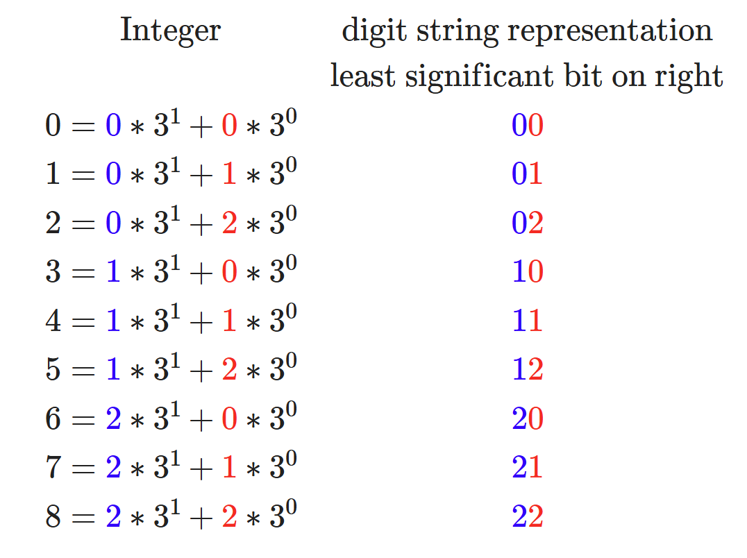
The statevector generated by the get_state command follows little-endian convention for associating numbers with their digit string representations, which places the least significant digit on the right. That is, for the example of a 2-qumode system of level 3 (in which possible states are 0, 1, and 2), resulting in the following translation between integers and digit string: