Quantum Fourier Transform¶

Classical Fourier transforms aid many areas such as signal processing and data compression. Below, we quantize it to enable Quantum Fourier Transforms (QFT) in CUDA-Q.

QFT is a key ingredient in Shor’s algorithm which is exponentially faster at factoring prime numbers and also plays a vital role in many other interesting quantum algorithms.

The idea with classical Fourier transforms is to take the problem from the frequency domain, to the time domain where it is easier to solve. This is the same analogy we draw with QFT, where we take the basis state from the computational basis to the Fourier basis.

The Quantum Fourier Transform is defined to be the linear operation which takes a basis state, \(\ket{x}\),

\[\begin{equation} \text{QFT}\ket{x} = \frac{1}{\sqrt{N}}\sum_{y=0}^{N-1} e^{\frac{2\pi ixy}{N}} \ket{y} \tag{1} \end{equation}\]

where \(n\) is the number of qubits and \(N= 2^n\).

It is convenient to represent states like \(\ket{x} = \ket{101}\) in their binary representation which in this case would be \(2^2 \times 1 + 2^1 \times 0 + 2^0 \times 1 = \ket{5}\).

For the \(n=1\) qubit case, we have the following basis states: \(\ket{0}, \ket{1}\). The QFT on these is as follows:

\[\begin{split}\begin{equation} \begin{aligned} \text{QFT}|0\rangle &= \frac{1}{\sqrt{2}}\sum_{y=0}^{2-1} e^{\frac{2\pi i(0)y}{2}}|y\rangle \\ &= \frac{1}{\sqrt{2}}\left(e^0|0\rangle + e^0|1\rangle\right) \\ &= \frac{1}{\sqrt{2}}(|0\rangle + |1\rangle) \\ &= \ket{+} \\ \end{aligned} \tag{2} \end{equation}\end{split}\]

\[\begin{split}\begin{equation} \begin{aligned} \text{QFT}|1\rangle &= \frac{1}{\sqrt{2}}\sum_{y=0}^{2-1} e^{\frac{2\pi i(1)y}{2}}|y\rangle \\ &= \frac{1}{\sqrt{2}}\left(e^0|0\rangle + e^{\pi i}|1\rangle\right) \\ &= \frac{1}{\sqrt{2}}(|0\rangle - |1\rangle) \\ &= \ket{-} \\ \end{aligned} \tag{3} \end{equation}\end{split}\]

To summarize, \(\text{QFT}|0\rangle = \ket{+}\) and \(\text{QFT}|1\rangle = \ket{-}\) which can be achieved by applying Hadamard gates.

Let us now extend this and see how we can apply this to \(n=3\) qubits.

For \(n=3, N = 2^3 = 8\) and we would like to perform \(\text{QFT}|101\rangle\) which in binary is \(2^2 \times 1 + 2^1 \times 0 + 2^0 \times 1 = 5\):

\[\begin{split}\begin{equation} \begin{aligned} \text{QFT}|101\rangle = \text{QFT}|5\rangle &= \frac{1}{\sqrt{8}}\sum_{y=0}^{8-1} e^{\frac{2\pi i(5)y}{8}}|y\rangle \\ &= \frac{1}{\sqrt{8}} [ e^{0}\ket{0} + e^{\frac{5i\pi (1)}{4}}\ket{1} + e^{\frac{5i\pi (2)}{4}}\ket{2} +...++ e^{\frac{5i\pi (7)}{4}}\ket{7} ] \\ &= \frac{1}{\sqrt{8}} [ \ket{000} + e^{\frac{5i\pi (1)}{4}}\ket{001} + e^{\frac{5i\pi (2)}{4}}\ket{010} +...++ e^{\frac{5i\pi (7)}{4}}\ket{111} ] \\ &= (0.35+0i) \ket{000} + (-0.25-0.25i)\ket{001} + (0+0.35i)\ket{010} +...+ (-0.25+0.25i)\ket{111} \\ \end{aligned} \tag{4} \end{equation}\end{split}\]

where we have used the fact that \(e^{i\theta} = \cos(\theta) + i\sin(\theta).\)

Here, we see how in addition to the Hadamard gates, we need some phase gates to apply the appropriate phases to the basis states. It turns out that the gate we need is the controlled \(R_k\) rotation where the \(R_k\) gate is denoted by:

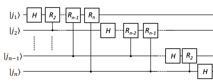
\[\begin{split}\begin{equation} R_k = \begin{bmatrix} 1 & 0 \\ 0 & e^{2\pi i/ 2^{k}} \end{bmatrix} \tag{5} \end{equation}\end{split}\]

Here is a generalized ciruit for a \(n\)-qubit quantum Fourier transform:

qft

Below we show the code for a QFT implementation in CUDA-Q based on the circuit diagram above:

[1]:

import cudaq
import numpy as np
from typing import List


@cudaq.kernel
def quantum_fourier_transform(input_state: List[int]):
    '''Args:
    input_state (list[int]): specifies the input state to be Fourier transformed.  '''

    qubit_count = len(input_state)

    # Initialize qubits.
    qubits = cudaq.qvector(qubit_count)

    # Initialize the quantum circuit to the initial state.
    for i in range(qubit_count):
        if input_state[i] == 1:
            x(qubits[i])

    # Apply Hadamard gates and controlled rotation gates.
    for i in range(qubit_count):
        h(qubits[i])
        for j in range(i + 1, qubit_count):
            angle = (2 * np.pi) / (2**(j - i + 1))
            cr1(angle, [qubits[j]], qubits[i])

[2]:

#Can be changed to 'nvidia' for single gpu, 'nvidia-mgpu' for multi-GPU or quantum hardware.
cudaq.set_target("qpp-cpu")

# The state to which the QFT operation is applied to. The zeroth element in the list is the zeroth qubit.
input_state = [1, 0, 1]

# Number of decimal points to round up the statevector to.
precision = 2

# Draw the quantum circuit.
print(cudaq.draw(quantum_fourier_transform, input_state))

# Print the statevector to the specified precision
statevector = np.array(cudaq.get_state(quantum_fourier_transform, input_state))
print(np.round(statevector, precision))

     ╭───╮╭───╮╭───────────╮╭────────────╮
q0 : ┤ x ├┤ h ├┤ r1(1.571) ├┤ r1(0.7854) ├───────────────────────
     ╰───╯╰───╯╰─────┬─────╯╰─────┬──────╯╭───╮╭───────────╮
q1 : ────────────────●────────────┼───────┤ h ├┤ r1(1.571) ├─────
     ╭───╮                        │       ╰───╯╰─────┬─────╯╭───╮
q2 : ┤ x ├────────────────────────●──────────────────●──────┤ h ├
     ╰───╯                                                  ╰───╯

[ 0.35+0.j   -0.25-0.25j  0.  +0.35j  0.25-0.25j -0.35+0.j    0.25+0.25j
 -0.  -0.35j -0.25+0.25j]

We can verify that this is the correct answer as above we worked out that:

\[\begin{split}\begin{equation} \begin{aligned} \text{QFT}|101\rangle = \text{QFT}|5\rangle &= \frac{1}{\sqrt{8}}\sum_{y=0}^{8-1} e^{\frac{2\pi i(5)y}{8}}|y\rangle \\ &= (0.35+0i) \ket{000} + (-0.25-0.25i)\ket{001} + (0+0.35i)\ket{010} +...+ (-0.25+0.25i)\ket{111}. \\ \end{aligned} \tag{6} \end{equation}\end{split}\]

Barring the gates used in the state preparation step, the circuit starts off by implementing a Hadamard gate and then \(n-1\) rotations on the zeroth qubit - a total of \(n\) gates. This is followed by a Hadamard and \(n-2\) conditional rotations on the first qubit which totals to \(n -1\) gates. If we continue the series, we get \(n + (n-1) + (n-2)... = n(n+1)/2\) gates. Hence, this circuit provides an algorithm with \(O(n^2)\) gates for computing the QFT.

The best classical algorithms for computing fast Fourier transforms on \(2^{n}\) elements require \(O(n2^{n})\) gates. This means that it requires exponentially more operations to compute the fast Fourier transform on a classical computer than it does to implement the QFT on a quantum computer.

Why are we not using QFT for real life applications then? The problem lies in quantum measurement. The quantum-Fourier-transformed amplitudes cannot be accessed by quantum measurement. However there are other quantum algorithms that do make use of QFT such as Shor’s algorithm.

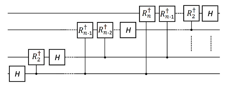
One can also invert the QFT where the circuit is executed in reverse with the inverse of each gate. The figure below shows the general \(n\)-qubit inverse QFT. Why don’t you try implementing this in CUDA-Q?

qft

Quantum Fourier Transform revisited¶

We provided one implementation of the Quantum Fourier Transform above. To demonstrate some of the other features of CUDA-Q, let’s define a new kernel for the Quantum Fourier Transform, which we’ll call quantum_fourier_transform2. Pay attention to how the kernel definition differs from the example above.

Since the Quantum Fourier Transform is a unitary operator, its inverse is its adjoint. Therefore, once we have implemented the Quantum Fourier Transform as a kernel in CUDA-Q, we can use the built-in adjoint operation to create the Inverse Quantum Fourier Transform.

[2]:

# Define kernels for the Quantum Fourier Transform and the Inverse Quantum Fourier Transform
@cudaq.kernel
def quantum_fourier_transform2(qubits: cudaq.qview):
    '''Args:
    qubits (cudaq.qview): specifies the quantum register to which apply the QFT.'''
    qubit_count = len(qubits)
    # Apply Hadamard gates and controlled rotation gates.
    for i in range(qubit_count):
        h(qubits[i])
        for j in range(i + 1, qubit_count):
            angle = (2 * np.pi) / (2**(j - i + 1))
            cr1(angle, [qubits[j]], qubits[i])


@cudaq.kernel
def inverse_qft(qubits: cudaq.qview):
    '''Args:
    qubits (cudaq.qview): specifies the quantum register to which apply the inverse QFT.'''
    cudaq.adjoint(quantum_fourier_transform2, qubits)

Let’s see that this approach gives us the same results as the section above.

[3]:

@cudaq.kernel
def verification_example(input_state: List[int]):
    '''Args:
    input_state (list[int]): specifies the input state to be transformed with QFT and the inverse QFT.  '''
    qubit_count = len(input_state)
    # Initialize qubits.
    qubits = cudaq.qvector(qubit_count)

    # Initialize the quantum circuit to the initial state.
    for i in range(qubit_count):
        if input_state[i] == 1:
            x(qubits[i])

    # Apply the quantum Fourier Transform
    quantum_fourier_transform2(qubits)

    # Apply the inverse quantum Fourier Transform
    inverse_qft(qubits)


# The state to which the QFT operation is applied to. The zeroth element in the list is the zeroth qubit.
input_state = [1, 0, 1]

# Number of decimal points to round up the statevector to.
precision = 2

print(cudaq.draw(verification_example, input_state))

# Print the statevector to the specified precision
statevector = np.array(cudaq.get_state(verification_example, input_state))
print(np.round(statevector, precision))  # The result should be the input state

     ╭───╮╭───╮╭─────────╮╭──────────╮                                      »
q0 : ┤ x ├┤ h ├┤ r1(1.5) ├┤ r1(0.75) ├──────────────────────────────────────»
     ╰───╯╰───╯╰────┬────╯╰────┬─────╯╭───╮╭─────────╮          ╭──────────╮»
q1 : ───────────────●──────────┼──────┤ h ├┤ r1(1.5) ├──────────┤ r1(-1.5) ├»
     ╭───╮                     │      ╰───╯╰────┬────╯╭───╮╭───╮╰────┬─────╯»
q2 : ┤ x ├─────────────────────●────────────────●─────┤ h ├┤ h ├─────●──────»
     ╰───╯                                            ╰───╯╰───╯            »

################################################################################

     ╭───────────╮╭──────────╮╭───╮
─────┤ r1(-0.75) ├┤ r1(-1.5) ├┤ h ├
╭───╮╰─────┬─────╯╰────┬─────╯╰───╯
┤ h ├──────┼───────────●───────────
╰───╯      │
───────────●───────────────────────


[0.+0.j 0.+0.j 0.+0.j 0.+0.j 0.+0.j 1.-0.j 0.-0.j 0.+0.j]

[3]:

print(cudaq.__version__)

CUDA-Q Version latest (https://github.com/NVIDIA/cuda-quantum a726804916fd397408cbf595ce6fe5f33dcd8b4c)