Multi-reference Quantum Krylov Algorithm - \(H_2\) Molecule
The multireference selected quantum Krylov (MRSQK) algorithm is defined in this paper and was developed as a low-cost alternative to quantum phase estimation. This tutorial will demonstrate how this algorithm can be implemented in CUDA-Q and accelerated using multiple GPUs. The CUDA-Q Hadamard test tutorial might provide helpful background information for understanding this tutorial.
The algorithm works by preparing an initial state, and then defining this state in a smaller subspace constructed with a basis that corresponds to Trotter steps of the initial state. This subspace can be diagonalized to produce an approximate energy for the system without variational optimization of any parameters.
In the example below, the initial guess is the ground state of the diagonalized Hamiltonian for demonstration purposes. In practice one could use a number of heuristics to prepare the ground state such as Hartree Fock or CISD. A very promising ground state preparation method which can leverage quantum computers is the linear combination of unitaries (LCU). LCU would allow for the state preparation to occur completely on the quantum computer and avoid storing an inputting the exponentially large state vector.
Regardless of the method used for state preparation, the procedure begins by selecting a \(d\)-dimensional basis of reference states \({\Phi_0 \cdots \Phi_d},\) where each is a linear combination of Slater determinants:
From this, a non-orthogonal Krylov Space \(\mathcal{K} = \{\psi_{0} \cdots \psi_{N}\}\) is constructed by applying a family of \(s\) unitary operators on each of the \(d\) reference states resulting in \(d*s = N\) elements in the Krylov space where
Therefore, the general quantum state that we originally set out to describe is
The energy of this state can be obtained by solving the generalized eigenvalue problem
where the elements of the overlap are
and Hamiltonian matrix is
The matrix elements for \(S\) are computed with the Hadamard test with a circuit shown below for the case of the overlap matrix elements.
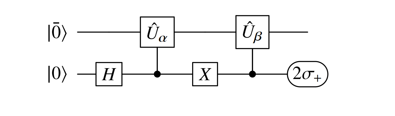
The \(2\sigma_+\) term refers to measurement of the expectation value of this circuit with the \(X+iY\) operator.
The Hamiltonian matrix elements are computed with a circuit that includes controlled application of the Hamiltonian. Once the \(H\) and \(S\) matrices are constructed, the diagonalization is performed classically to produce an estimate for the ground state in question.
Setup
This cell installs the necessary packages.
[1]:
%pip install pyscf
import cudaq
import numpy as np
import scipy

# Single-node, single gpu
if cudaq.num_available_gpus() > 0 and cudaq.has_target("nvidia"):
    cudaq.set_target("nvidia")
else:
    print("CUDA or GPU support is unavailable. Running with CPU simulator. Performance may be significantly reduced.")
    cudaq.set_target("qpp-cpu")
The molecule is defined below and its Hamiltonian is extracted as a matrix. The matrix is diagonalized to produce the ground state. The corresponding state vector will be used as the initial state to ensure good results for this demonstration.
[2]:
from qchem.classical_pyscf import get_mol_hamiltonian
from qchem.hamiltonian import jordan_wigner_fermion

# Define H2 molecule

# Generate the spin Hamiltonian

geometry = 'H 0.0 0.0 0.0; H 0.0 0.0 0.7474'
#geometry = 'Li 0.3925 0.0 0.0; H -1.1774 0.0 0.0'
#geometry = "qchem/H2O.xyz"


# Run HF, ccsd and compute the spin molecular hamiltonian using the HF molecular orbitals.
molecular_data = get_mol_hamiltonian(xyz=geometry, spin=0, charge=0, basis='sto3g', ccsd=True, verbose=True)

# For active space calculations, we can specify the number of active electrons and orbitals.
#molecular_data = get_mol_hamiltonian(xyz=geometry, spin=0, charge=0, basis='631g', nele_cas=4, norb_cas=4,
#                                     ccsd=True, casci=True, verbose=True)

obi = molecular_data[0]
tbi = molecular_data[1]
e_nn = molecular_data[2]
nelectrons = molecular_data[3]
norbitals = molecular_data[4]

qubits_num = 2 * norbitals

# Jordan-Wigner transformation to convert the fermionic Hamiltonian to a spin Hamiltonian
hamiltonian = jordan_wigner_fermion(obi, tbi, e_nn, tolerance = 1e-12)

# Diagonalize Hamiltonian
spin_ham_matrix = hamiltonian.to_matrix()
e, c = np.linalg.eig(spin_ham_matrix)

# Find the ground state energy and the corresponding eigenvector
print('Ground state energy (classical simulation)= ', np.min(e), ', index= ',
      np.argmin(e))
min_indices = np.argmin(e)

# Eigenvector can be used to initialize the qubits
vec = c[:, min_indices]
overwrite output file: H 0-pyscf.log
[pyscf] Total number of orbitals =  2
[pyscf] Total number of electrons =  2
[pyscf] HF energy =  -1.116325564486115
[pyscf] Total R-CCSD energy =  -1.1371758844013327
Ground state energy (classical simulation)=  (-1.1371757102406845+0j) , index=  3
The functions below take the original Hamiltonian defined above, and strip it into a list of Pauli words and a list of coefficients which will be uses later.
[3]:
# Collect coefficients from a spin operator so we can pass them to a kernel.
# The identity term is excluded. Its contribution is added back to the
# Hamiltonian matrix classically below.
def term_coefficients(ham: cudaq.SpinOperator) -> list[complex]:
    result = []
    for term in ham:
        if term.is_identity():
            continue
        result.append(term.evaluate_coefficient())
    return result

# Collect Pauli words from a spin operator so we can pass them to a kernel
def term_words(ham: cudaq.SpinOperator) -> list[str]:
    # Our kernel uses these words to apply exp_pauli to the entire state.
    # we hence ensure that each pauli word covers the entire space.
    result = []
    for term in ham:
        if term.is_identity():
            continue
        result.append(term.get_pauli_word(qubits_num))
    return result

# Build the lists of coefficients and Pauli Words from the H2 Hamiltonian
coefficient = term_coefficients(hamiltonian)
pauli_string = term_words(hamiltonian)

# Sum of identity-term coefficients
# The identity contributes `identity_coef * S` to the Hamiltonian matrix.
identity_coef = sum(
    term.evaluate_coefficient().real
    for term in hamiltonian
    if term.is_identity())

print(coefficient)
print(pauli_string)
[(0.17028010135220506+0j), (0.17028010135220503+0j), (-0.2200413002242175+0j), (-0.2200413002242175+0j), (0.1683359862516207+0j), (0.12020049071260122+0j), (0.1656068235817425+0j), (0.1656068235817425+0j), (0.12020049071260122+0j), (0.17407289249680213+0j), (-0.04540633286914128+0j), (0.04540633286914128+0j), (0.04540633286914128+0j), (-0.04540633286914128+0j)]
['ZIII', 'IZII', 'IIZI', 'IIIZ', 'ZZII', 'ZIZI', 'ZIIZ', 'IZZI', 'IZIZ', 'IIZZ', 'XXYY', 'XYYX', 'YXXY', 'YYXX']
In this example, the unitary operators that build the Krylov subspace are first-order Trotter operations at different time steps. The performance here could potentially be improved by increasing the size of the time step, using a higher order Trotter approximation, or using other sorts of approximations. The CUDA-Q kernels below define the unitary operations that construct the \(\psi\) basis. Each receives the target qubits, the time step, and components of the Hamiltonian.
[4]:
# Applies Unitary operation corresponding to Um
@cudaq.kernel
def U_m(qubits: cudaq.qview, dt: float, coefficients: list[complex],
        words: list[cudaq.pauli_word]):
    # Compute U_m = exp(-i m dt H)
    for i in range(len(coefficients)):
        exp_pauli(dt * coefficients[i].real, qubits, words[i])


# Applies Unitary operation corresponding to Un


@cudaq.kernel
def U_n(qubits: cudaq.qview, dt: float, coefficients: list[complex],
        words: list[cudaq.pauli_word]):
    # Compute U_n = exp(-i n dt H)
    for i in range(len(coefficients)):
        exp_pauli(dt * coefficients[i].real, qubits, words[i])


# Applies the gate operations for a Hamiltonian Pauli Word


@cudaq.kernel
def apply_pauli(qubits: cudaq.qview, word: list[int]):
    # Add H (Hamiltonian operator)
    for i in range(len(word)):
        if word[i] == 1:
            x(qubits[i])
        if word[i] == 2:
            y(qubits[i])
        if word[i] == 3:
            z(qubits[i])


# Performs Hadamard test circuit which determines matrix elements of S and H of subspace


@cudaq.kernel
def qfd_kernel(dt_alpha: float, dt_beta: float, coefficients: list[complex],
               words: list[cudaq.pauli_word], word_list: list[int],
               vec: list[complex]):

    ancilla = cudaq.qubit()
    qreg = cudaq.qvector(vec)

    h(ancilla)

    x(ancilla)
    cudaq.control(U_m, ancilla, qreg, dt_alpha, coefficients, words)
    x(ancilla)

    cudaq.control(apply_pauli, ancilla, qreg, word_list)
    cudaq.control(U_n, ancilla, qreg, dt_beta, coefficients, words)
The auxillary function below takes a Pauli word, and converts it to a list of integers which informs applications of this word to a circuit with the apply_pauli kernel.
[5]:
def pauli_str(pauli_word, qubits_num):

    my_list = []
    for i in range(qubits_num):
        if str(pauli_word[i]) == 'I':
            my_list.append(0)
        if str(pauli_word[i]) == 'X':
            my_list.append(1)
        if str(pauli_word[i]) == 'Y':
            my_list.append(2)
        if str(pauli_word[i]) == 'Z':
            my_list.append(3)
    return my_list
The spin operators necessary for the Hadamard test are defined below.
[6]:
# Define the spin-op x for real component and y for the imaginary component.
x_0 = cudaq.spin.x(0)
y_0 = cudaq.spin.y(0)
Finally, the time step for the unitary operations that build the Krylov space is defined as well as the dimension of the Krylov space.
[7]:
#Define parameters for the quantum Krylov space
dt = 0.5

# Dimension of the Krylov space
m_qfd = 4
Computing the matrix elements
The cell below computes the overlap matrix. This can be done in serial or in parallel, depending on the multi_gpu specification. First, an operator is built to apply the identity to the overlap matrix circuit when apply_pauli is called. Next, the wf_overlap array is constructed which will hold the matrix elements.
Next, a pair of nested loops iterate over the time steps defined by the dimension of the subspace. Each m,n combination corresponds to computation of an off-diagonal matrix element of the overlap matrix \(S\) using the Hadamard test. This is accomplished by calling the CUDA-Q observe function with the X and Y operators, along with the time steps, the components of the Hamiltonian matrix, and the initial state vector vec.
The observe function broadcasts over the two provided operators \(X\) and \(Y\) and returns a list of results. The expectation function returns the expectation values which are summed and stored in the matrix.
The multi-gpu case completes the same steps, except the observe_async command is used. This allows for the \(X\) and \(Y\) observables to be evaluated at the same time on two different simulated QPUs. In this case, the results are stored in lists corresponding to the real and imaginary parts. These are then accessed later with the get command to build \(S\).
[8]:
# Create the identity operator
identity_op = cudaq.SpinOperator.from_word('I' * qubits_num)
# Get the Pauli word and convert it to a list of integers
# where I=0, X=1, Y=2, Z=3
# This is used to apply the identity operator in the kernel.
identity_word = identity_op.get_pauli_word()
pauli_list = pauli_str(identity_word, qubits_num)

# Empty overlap matrix S
wf_overlap = np.zeros((m_qfd, m_qfd), dtype=complex)
# Loop to solve for S matrix elements
for m in range(m_qfd):
    dt_m = dt * m
    for n in range(m, m_qfd):
        dt_n = dt * n
        results = cudaq.observe(qfd_kernel, [x_0, y_0], dt_m, dt_n,
                                coefficient, pauli_string, pauli_list, vec)
        temp = [result.expectation() for result in results]
        wf_overlap[m, n] = temp[0] + temp[1] * 1j
        if n != m:
            wf_overlap[n, m] = np.conj(wf_overlap[m, n])
The Hamiltonian matrix elements are computed in the same way, except this time the Hamiltonian is applied as part of the circuit. This is accomplished with the extra for loop, which iterates through the terms in the Hamiltonian, computing an expectation value for each one and then summing the results to produce one matrix element.
[9]:
## Single GPU:

# Empty H matrix
# This matrix will be used to store the Hamiltonian matrix elements
# for the Krylov subspace.
# The matrix is symmetric, so we only need to compute the upper triangle.
# The matrix is of size m_qfd x m_qfd, where m_qfd is the dimension of the Krylov subspace.
ham_matrx = np.zeros((m_qfd, m_qfd), dtype=complex)

# Loops over H matrix terms
for m in range(m_qfd):
    dt_m = dt * m
    for n in range(m, m_qfd):
        dt_n = dt * n

        # 2 entry array that stores real and imaginary part of matrix element
        tot_e = np.zeros(2)

        # Loops over the (non-identity) terms in the Hamiltonian, computing expectation values
        for coef, word in zip(coefficient, pauli_string):
            pauli_list = pauli_str(word, qubits_num)

            results = cudaq.observe(qfd_kernel, [x_0, y_0], dt_m, dt_n,
                                        coefficient, pauli_string, pauli_list,
                                        vec)

            temp = [result.expectation() for result in results]

            # Multiplies result by coefficient corresponding to Pauli Word
            temp[0] = coef.real * temp[0]
            temp[1] = coef.real * temp[1]

            # Accumulates results for each Pauli Word
            tot_e[0] += temp[0]
            tot_e[1] += temp[1]

        # Adds back the identity-term contribution.
        ham_matrx[m, n] = tot_e[0] + tot_e[1] * 1j + identity_coef * wf_overlap[m, n]
        if n != m:
            ham_matrx[n, m] = np.conj(ham_matrx[m, n])
Determining the ground state energy of the subspace
The final step is to solve the generalized eigenvaulue problem with the overlap and Hamiltonian matrices constructed using the quantum computer. The procedure begins by diagonalizing \(S\) with the transform
The eigenvectors \(v\) and eigenvalues \(s\) are used to construct a new matrix \(X':\)
The matrix \(X'\) diagonalizes \(H:\)
Using the eigenvectors of \(H'\), (\(^{\frac{1}{2}}C\)), the original eigenvectors to the problem can be found by left multiplying by \(S^{\frac{-1}{2}}C.\)
[10]:
def eig(H, s):
    #Solver for generalized eigenvalue problem
    # HC = SCE

    THRESHOLD = 1e-20
    s_diag, u = scipy.linalg.eig(s)
    s_prime = []
    for sii in s_diag:
        if np.imag(sii) > 1e-7:
            raise ValueError(
                "S may not be hermitian, large imag. eval component.")
        if np.real(sii) > THRESHOLD:
            s_prime.append(np.real(sii))

    X_prime = np.zeros((len(s_diag), len(s_prime)), dtype=complex)

    for i in range(len(s_diag)):
        for j in range(len(s_prime)):
            X_prime[i][j] = u[i][j] / np.sqrt(s_prime[j])

    H_prime = (((X_prime.conjugate()).transpose()).dot(H)).dot(X_prime)
    e_prime, C_prime = scipy.linalg.eig(H_prime)
    C = X_prime.dot(C_prime)

    return e_prime, C
[11]:
eigen_value, eigen_vect = eig(ham_matrx[0:m_qfd, 0:m_qfd], wf_overlap[0:m_qfd,
                                                                      0:m_qfd])
print('Energy from QFD:')
print(np.min(eigen_value))
Energy from QFD:
(-1.1359686811350462-4.497484607599205e-09j)