Using the Hadamard Test to Determine Quantum Krylov Subspace Decomposition Matrix Elements
The Hadamard test is a quantum algorithm for estimating expectation values and is a useful subroutine for a number of quantum applications ranging from estimation of molecular ground state energies to quantum semidefinite programming. This tutorial will briefly introduce the Hadamard test, demonstrate how it can be implemented in CUDA-Q, and then parallelized for a Quantum Krylov Subspace Diagonalization application.
The Hadamard test is performed using a register with an ancilla qubit in the \(\ket{0}\) state and a prepared quantum state \(\ket{\psi}\), the following circuit can be used to extract the expectation value from measurement of the ancilla.
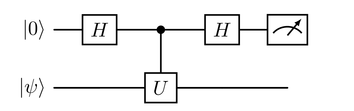
The key insight is that
and
so their difference is equal to
More details and a short derivation can be found here.
What if you want to perform the Hadamard test to compute an expectation value like \(\bra{\psi} O \ket{\phi}\), where \(\ket{\psi}\) and \(\ket{\phi}\) are different states and \(O\) is a Pauli Operator? This is a common subroutine for the QKSD, where matrix elements are determined by computing expectation values between different states.
Defining \(O\) as
and given the fact that
we can combine the state preparation steps into the operator resulting in
which corresponds to the following circuit. 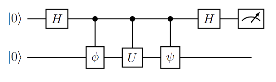
By preparing this circuit, and repeatedly measuring the ancilla qubit, we estimate the expectation value as
The following sections demonstrate how this can be performed in CUDA-Q.
Numerical result as a reference:
Before performing the Hadamard test, let’s determine the exact expectation value by performing the matrix multiplications explicitly. The code below builds two CUDA-Q kernels corresponding to \(\ket{\psi} = \frac{1}{\sqrt{2}}\begin{pmatrix}1 \\ 0 \\ 1 \\ 0\end{pmatrix}\) and \(\ket{\phi} = \begin{pmatrix}0 \\ 1 \\ 0 \\ 0\end{pmatrix}.\)
[1]:
import cudaq
import numpy as np
from functools import reduce

if cudaq.num_available_gpus() > 0 and cudaq.has_target("nvidia"):
    cudaq.set_target("nvidia")
else:
    print("CUDA or GPU support is unavailable. Running with CPU simulator. Performance may be significantly reduced.")
    cudaq.set_target("qpp-cpu")

qubit_num = 2


@cudaq.kernel
def psi(num: int):
    q = cudaq.qvector(num)
    h(q[1])


@cudaq.kernel
def phi(n: int):
    q = cudaq.qvector(n)
    x(q[0])
The state vectors can be accessed using the get_state command and printed as numpy arrays:
[2]:
psi_state = cudaq.get_state(psi, qubit_num)
print('Psi state: ', psi_state)

phi_state = cudaq.get_state(phi, qubit_num)
print('Phi state: ', phi_state)
Psi state:  (0.707107,0)
(0,0)
(0.707107,0)
(0,0)

Phi state:  (0,0)
(1,0)
(0,0)
(0,0)
The Hamiltonian operator (\(O\) in the derivation above) is defined as a CUDA-Q spin operator and converted to a matrix with to_matrix. The following line of code performs the explicit matrix multiplications to produce the exact expectation value.
[3]:
ham = cudaq.spin.x(0) * cudaq.spin.x(1)
ham_matrix = ham.to_matrix()
print('hamiltonian: ', np.array(ham_matrix), '\n')

exp_val = reduce(np.dot, (np.array(psi_state).conj().T, ham_matrix, phi_state))

print('Numerical expectation value: ', exp_val)
hamiltonian:  [[0.+0.j 0.+0.j 0.+0.j 1.+0.j]
 [0.+0.j 0.+0.j 1.+0.j 0.+0.j]
 [0.+0.j 1.+0.j 0.+0.j 0.+0.j]
 [1.+0.j 0.+0.j 0.+0.j 0.+0.j]]

Numerical expectation value:  (0.7071067690849304+0j)
Using Sample to perform the Hadamard test
Three CUDA-Q kernels are constructed below corresponding to \(\ket{\psi}\), \(\ket{\phi}\), and the Hamiltonian. A fourth kernel constructs the Hadamard test circuit and completes with a measurement of the ancilla qubit in the computational basis.
[4]:
import cudaq

if cudaq.num_available_gpus() > 0 and cudaq.has_target("nvidia"):
    cudaq.set_target("nvidia")
else:
    print("CUDA or GPU support is unavailable. Running with CPU simulator. Performance may be significantly reduced.")
    cudaq.set_target("qpp-cpu")


@cudaq.kernel
def U_psi(q: cudaq.qview):
    h(q[1])


@cudaq.kernel
def U_phi(q: cudaq.qview):
    x(q[0])


@cudaq.kernel
def ham_cir(q: cudaq.qview):
    x(q[0])
    x(q[1])


@cudaq.kernel
def kernel(n: int):
    ancilla = cudaq.qubit()
    q = cudaq.qvector(n)
    h(ancilla)
    cudaq.control(U_phi, ancilla, q)
    cudaq.control(ham_cir, ancilla, q)
    cudaq.control(U_psi, ancilla, q)

    h(ancilla)

    mz(ancilla)
The CUDA-Q sample method computes 100000 sample ancilla measurements, and from them we can estimate the expectation value. The standard error is provided as well. Try increasing the sample size and note the convergence of the expectation value and the standard error towards the numerical result.
[5]:
shots = 100000
qubit_num = 2
count = cudaq.sample(kernel, qubit_num, shots_count=shots)
print(count)

mean_val = (count['0'] - count['1']) / shots
error = np.sqrt(2 * count['0'] * count['1'] / shots) / shots
print('Observable QC: ', mean_val, '+ -', error)
print('Numerical result', np.real(exp_val))
{ 0:85509 1:14491 }

Observable QC:  0.71018 + - 0.0015742369065677502
Numerical result 0.7071067690849304
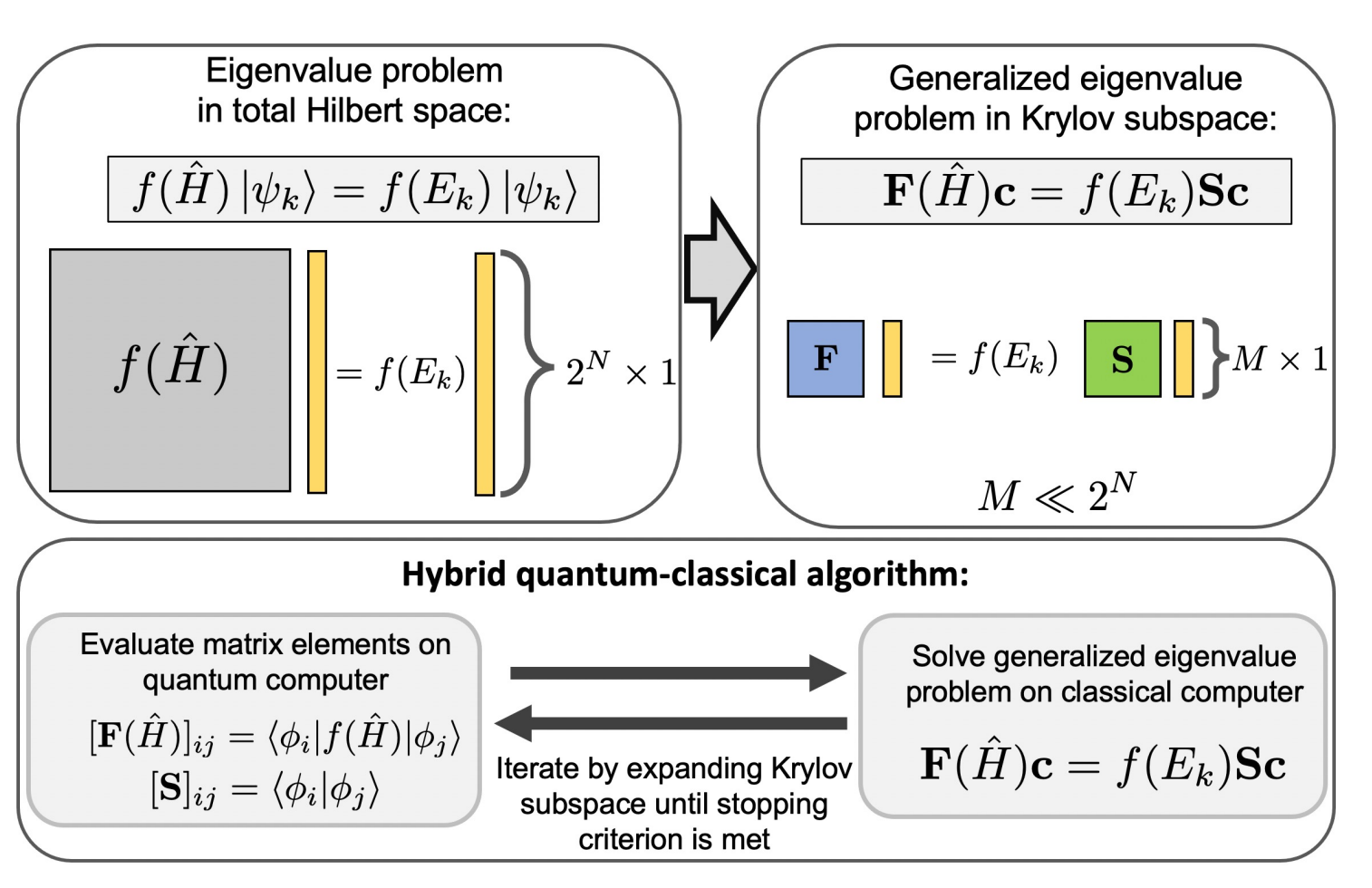
Multi-GPU evaluation of QKSD matrix elements using the Hadamard Test
This example is small, but a more practical application of the Hadamard test such as QKSD will require much larger circuits. The QKSD method works by reducing the exponential \(2^N\) Hilbert space into an exponentially smaller subspace using a set of non-orthogonal states which are easy to prepare on a quantum computer. The Hadamard test is used to compute the matrix elements of this smaller subspace which is then diagonalized using a classical method to produce the eigenvalues. This paper described the method in more detail and is the source of the figure below.
This method can be easily parallelized, and multiple QPUs, if available, could compute the matrix elements asynchronously. The CUDA-Q mqpu backend allows you to simulate a computation across multiple simulated QPUs. The code below demonstrates how.
First, the Hadamard test circuit is defined, but this time the \(\ket{\psi}\) and \(\ket{\phi}\) states contain parameterized rotations so that multiple states can be quickly generated, for the sake of example.
[6]:
import cudaq


@cudaq.kernel
def U_psi(q: cudaq.qview, theta: float):
    ry(theta, q[1])


@cudaq.kernel
def U_phi(q: cudaq.qview, theta: float):
    rx(theta, q[0])


@cudaq.kernel
def ham_cir(q: cudaq.qview):
    x(q[0])
    x(q[1])


@cudaq.kernel
def kernel(n: int, angle: float, theta: float):
    ancilla = cudaq.qubit()
    q = cudaq.qvector(n)
    h(ancilla)
    cudaq.control(U_phi, ancilla, q, theta)
    cudaq.control(ham_cir, ancilla, q)
    cudaq.control(U_psi, ancilla, q, angle)

    h(ancilla)

    mz(ancilla)
Next, the nvidia-mqpu backend is specified and the number of GPUs available is determined.
[7]:
if cudaq.num_available_gpus() > 1 and cudaq.has_target("nvidia"):
    cudaq.set_target("nvidia", option="mqpu")
elif cudaq.num_available_gpus() > 0 and cudaq.has_target("nvidia"):
    cudaq.set_target("nvidia")
else:
    print("CUDA or GPU support is unavailable. Running with CPU simulator. Performance may be significantly reduced.")
    cudaq.set_target("qpp-cpu")

target = cudaq.get_target()
qpu_count = target.num_qpus()
print("Number of QPUs:", qpu_count)
Number of QPUs: 1
The sample_async command is then used to distribute the Hadamard test computations across multiple simulated QPUs. The results are saved in a list and accessed below.
[8]:
shots = 100000
angle = [0.0, 1.5, 3.14, 0.7]
theta = [0.6, 1.2, 2.2, 3.0]
qubit_num = 2

result = []
for i in range(4):
    count = cudaq.sample_async(kernel,
                               qubit_num,
                               angle[i],
                               theta[i],
                               shots_count=shots,
                               qpu_id=i % qpu_count)
    result.append(count)
The four matrix elements are shown below and can be classically processed to produce the eigenvalues.
[9]:
mean_val = np.zeros(len(angle))
i = 0
for count in result:
    print(i)
    i_result = count.get()
    print(i_result)
    mean_val[i] = (i_result['0'] - i_result['1']) / shots
    error = np.sqrt(2 * i_result['0'] * i_result['1'] / shots) / shots
    print('QKSD Matrix Element: ', mean_val[i], '+ -', error)
    i += 1
0
{ 0:49880 1:50120 }

QKSD Matrix Element:  -0.0024 + - 0.002236061537614741
1
{ 0:50111 1:49889 }

QKSD Matrix Element:  0.00222 + - 0.0022360624673742903
2
{ 0:50127 1:49873 }

QKSD Matrix Element:  0.00254 + - 0.0022360607643800738
3
{ 0:49832 1:50168 }

QKSD Matrix Element:  -0.00336 + - 0.0022360553553076455
Classically Diagonalize the Subspace Matrix
For a problem of this size, numpy can be used to diagonalize the subspace and produce the eigenvalues and eigenvectors in the basis of non-orthogonal states.
[10]:
import numpy as np

my_mat = np.zeros((2, 2), dtype=float)
m = 0
for k in range(2):
    for j in range(2):
        my_mat[k, j] = mean_val[m]
        m += 1

print(my_mat)

E, V = np.linalg.eigh(my_mat)

print('Eigenvalues: ')
print(E)

print('Eigenvector: ')
print(V)
[[-0.0024   0.00222]
 [ 0.00254 -0.00336]]
Eigenvalues:
[-0.00546496 -0.00029504]
Eigenvector:
[[-0.63808707 -0.76996421]
 [ 0.76996421 -0.63808707]]