Control

These examples all cover dynamical simulation of systems related to device control. These examples use small systems, but note that the GPU will only provide an advantage for systems with total dimension of O(1000).

Gate Calibration

This example demonstrates how to perform pulse optimization.

import cudaq
from cudaq import boson, Schedule, ScalarOperator, ScipyZvodeIntegrator
import numpy as np
import cupy as cp
import os
import matplotlib.pyplot as plt

# Set the target to our dynamics simulator
cudaq.set_target("dynamics")

# Sample device parameters
# Assuming a simple transmon device Hamiltonian in rotating frame.
detuning = 0.0  # Detuning of the drive; assuming resonant drive
anharmonicity = -340.0  # Anharmonicity
sigma = 0.01  # sigma of the Gaussian pulse
cutoff = 4.0 * sigma  # total length of drive pulse

# Dimensions of sub-system
# We model `transmon` as a 3-level system to account for leakage.
dimensions = {0: 3}

# Initial state of the system (ground state).
psi0 = cudaq.State.from_data(cp.array([1.0, 0.0, 0.0], dtype=cp.complex128))


def gaussian(t):
    """
    Gaussian shape with cutoff. Starts at t = 0, amplitude normalized to one
    """
    val = (np.exp(-((t-cutoff/2)/sigma)**2/2)-np.exp(-(cutoff/sigma)**2/8)) \
           / (1-np.exp(-(cutoff/sigma)**2/8))
    return val


def dgaussian(t):
    """
    Derivative of Gaussian. Starts at t = 0, amplitude normalized to one
    """
    return -(t - cutoff / 2) / sigma * np.exp(-(
        (t - cutoff / 2) / sigma)**2 / 2 + 0.5)


# Schedule of time steps.
steps = np.linspace(0.0, cutoff, 201)
schedule = Schedule(steps, ["t"])

# We optimize for a X(pi/2) rotation
target_state = np.array([1.0 / np.sqrt(2), -1j / np.sqrt(2), 0.0],
                        dtype=cp.complex128)


# Optimize the amplitude of the drive pulse (DRAG - Derivative Removal by Adiabatic Gate)
def cost_function(amps):
    amplitude = 100 * amps[0]
    drag_amp = 100 * amps[1]
    # Qubit Hamiltonian
    hamiltonian = detuning * boson.number(0) + (
        anharmonicity / 2) * boson.create(0) * boson.create(
            0) * boson.annihilate(0) * boson.annihilate(0)
    # Drive term
    hamiltonian += amplitude * ScalarOperator(gaussian) * (boson.create(0) +
                                                           boson.annihilate(0))

    # Drag term (leakage reduction)
    hamiltonian += 1j * drag_amp * ScalarOperator(dgaussian) * (
        boson.annihilate(0) - boson.create(0))

    # We optimize for a X(pi/2) rotation
    evolution_result = cudaq.evolve(hamiltonian,
                                    dimensions,
                                    schedule,
                                    psi0,
                                    observables=[],
                                    collapse_operators=[],
                                    store_intermediate_results=cudaq.IntermediateResultSave.NONE,
                                    integrator=ScipyZvodeIntegrator())
    final_state = evolution_result.final_state()

    overlap = np.abs(final_state.overlap(target_state))
    print(
        f"Gaussian amplitude = {amplitude}, derivative amplitude = {drag_amp}, Overlap: {overlap}"
    )
    return 1.0 - overlap


# Specify the optimizer
optimizer = cudaq.optimizers.NelderMead()
optimal_error, optimal_parameters = optimizer.optimize(dimensions=2,
                                                       function=cost_function)

print("optimal overlap =", 1.0 - optimal_error)
print("optimal parameters =", optimal_parameters)

Gaussian amplitude = 0.0, derivative amplitude = 0.0, Overlap: 0.7071067811865475
Gaussian amplitude = 157.07963267948966, derivative amplitude = 0.0, Overlap: 0.7678402941325417
Gaussian amplitude = 157.07963267948966, derivative amplitude = 157.07963267948966, Overlap: 0.6797941803182259
Gaussian amplitude = 0.0, derivative amplitude = -157.07963267948966, Overlap: 0.9296240579072232
Gaussian amplitude = -78.53981633974483, derivative amplitude = -314.1592653589793, Overlap: 0.7162211356808167
Gaussian amplitude = 157.07963267948966, derivative amplitude = -157.07963267948966, Overlap: 0.44596190760545296
Gaussian amplitude = 39.269908169872416, derivative amplitude = -39.269908169872416, Overlap: 0.9398996786747706
Gaussian amplitude = -117.80972450961724, derivative amplitude = -196.34954084936206, Overlap: 0.5878521963356885
Gaussian amplitude = 88.35729338221293, derivative amplitude = -49.087385212340514, Overlap: 0.6575502829271433
Gaussian amplitude = 98.17477042468103, derivative amplitude = -19.634954084936208, Overlap: 0.33247544702132076
Gaussian amplitude = 19.634954084936208, derivative amplitude = -98.17477042468103, Overlap: 0.8409827814368478
Gaussian amplitude = -39.269908169872416, derivative amplitude = -117.80972450961724, Overlap: 0.9445817360291182
Gaussian amplitude = -107.99224746714913, derivative amplitude = -166.89710972195778, Overlap: 0.7586919940233878
Gaussian amplitude = -19.634954084936208, derivative amplitude = -58.90486225480862, Overlap: 0.7406581261969767
Gaussian amplitude = 9.817477042468104, derivative amplitude = -88.35729338221293, Overlap: 0.8651921848480539
Gaussian amplitude = -9.817477042468104, derivative amplitude = -68.72233929727672, Overlap: 0.8181626678528717
Gaussian amplitude = 4.908738521234052, derivative amplitude = -83.44855486097889, Overlap: 0.8663447451357891
Gaussian amplitude = -4.908738521234052, derivative amplitude = -73.63107781851078, Overlap: 0.8433090770060998
Gaussian amplitude = 2.454369260617026, derivative amplitude = -80.99418560036186, Overlap: 0.8638676425264983
Gaussian amplitude = 0.0, derivative amplitude = -78.53981633974483, Overlap: 0.8592468550642993
Gaussian amplitude = -17.18058482431918, derivative amplitude = -100.62913968529807, Overlap: 0.9218675201964192
Gaussian amplitude = -56.45049299419159, derivative amplitude = -139.8990478551705, Overlap: 0.9265972065467258
Gaussian amplitude = -78.53981633974483, derivative amplitude = -157.07963267948966, Overlap: 0.835400572144582
Gaussian amplitude = -32.520392703175595, derivative amplitude = -114.74176293384598, Overlap: 0.9480750666520233
Gaussian amplitude = -15.339807878856416, derivative amplitude = -92.65243958829275, Overlap: 0.9007114410060454
Gaussian amplitude = -46.1728217153578, derivative amplitude = -128.08739578845106, Overlap: 0.9490749424029333
Gaussian amplitude = -39.42330624866097, derivative amplitude = -125.0194342126798, Overlap: 0.9590912872207543
Gaussian amplitude = -39.50000528805525, derivative amplitude = -128.6242890642111, Overlap: 0.9644209828123245
Gaussian amplitude = -53.15243430023746, derivative amplitude = -141.96992191881617, Overlap: 0.9371109174510482
Gaussian amplitude = -37.67840310244106, derivative amplitude = -121.54880268008851, Overlap: 0.9556739509139307
Gaussian amplitude = -31.005586675138513, derivative amplitude = -122.08569595584855, Overlap: 0.9654586085651646
Gaussian amplitude = -23.421969155028872, derivative amplitude = -119.0848460395473, Overlap: 0.963623453294681
Gaussian amplitude = -32.82718886075271, derivative amplitude = -129.1611823399711, Overlap: 0.9745284542544127
Gaussian amplitude = -30.401581739908533, derivative amplitude = -132.9673721699124, Overlap: 0.9801467465441793
Gaussian amplitude = -21.9071631269918, derivative amplitude = -126.42877906154987, Overlap: 0.9754292788007772
Gaussian amplitude = -21.303158191761824, derivative amplitude = -137.31045527561375, Overlap: 0.9831092973124017
Gaussian amplitude = -16.451943950073478, derivative amplitude = -144.92283493549633, Overlap: 0.9767359198754701
Gaussian amplitude = -29.79757680467855, derivative amplitude = -143.84904838397628, Overlap: 0.9800104018090544
Gaussian amplitude = -27.82497338525686, derivative amplitude = -139.49398105336968, Overlap: 0.983130133355889
Gaussian amplitude = -18.726549837110152, derivative amplitude = -143.83706415907102, Overlap: 0.9795024686649386
Gaussian amplitude = -27.48282376420894, derivative amplitude = -135.68479516720205, Overlap: 0.9830113579207141
Gaussian amplitude = -21.645307812809744, derivative amplitude = -141.11964116178137, Overlap: 0.9826376028076026
Gaussian amplitude = -26.02344477635914, derivative amplitude = -137.0435066658469, Overlap: 0.9836739278237355
Gaussian amplitude = -32.545259969854186, derivative amplitude = -139.2270324436028, Overlap: 0.9801447148031301
Gaussian amplitude = -24.113683636284915, derivative amplitude = -137.78959956761102, Overlap: 0.9838140571803666
Gaussian amplitude = -22.31215502738719, derivative amplitude = -135.33912518008825, Overlap: 0.9830417565995295
Gaussian amplitude = -26.446768795789446, derivative amplitude = -138.45526708504931, Overlap: 0.9836520843944795
Gaussian amplitude = -23.690359616854607, derivative amplitude = -136.3778391484086, Overlap: 0.9836030636444814
Gaussian amplitude = -25.75766650105573, derivative amplitude = -137.93591010088915, Overlap: 0.9837756871844154
Gaussian amplitude = -23.847905360981503, derivative amplitude = -138.68200300265326, Overlap: 0.9837642033752482
Gaussian amplitude = -24.39179021482591, derivative amplitude = -138.27237891845166, Overlap: 0.9838287992237971
Gaussian amplitude = -22.747807350055094, derivative amplitude = -138.12606838517354, Overlap: 0.983605007962648
Gaussian amplitude = -25.00520171330557, derivative amplitude = -137.98344967196024, Overlap: 0.9838349659123633
Gaussian amplitude = -25.283308291846573, derivative amplitude = -138.46622902280092, Overlap: 0.9838084449662036
Gaussian amplitude = -24.40608980017533, derivative amplitude = -137.9587569314085, Overlap: 0.9838333961345107
Gaussian amplitude = -25.01950129865499, derivative amplitude = -137.6698276849171, Overlap: 0.9838262991248778
Gaussian amplitude = -24.54871798578318, derivative amplitude = -138.12174111006803, Overlap: 0.9838371837908917
Gaussian amplitude = -25.14782989891342, derivative amplitude = -138.14643385061981, Overlap: 0.9838281816540192
Gaussian amplitude = -24.59152482485985, derivative amplitude = -138.0056761612113, Overlap: 0.9838386325114293
Gaussian amplitude = -24.135041097337464, derivative amplitude = -138.1439675993191, Overlap: 0.9838178216495735
Gaussian amplitude = -24.78766155931354, derivative amplitude = -138.02357915379997, Overlap: 0.9838394947681391
Gaussian amplitude = -24.83046839839021, derivative amplitude = -137.90751420494328, Overlap: 0.9838382084236699
Gaussian amplitude = -24.760030795238453, derivative amplitude = -137.96107093122444, Overlap: 0.983839415811919
Gaussian amplitude = -24.95616752969215, derivative amplitude = -137.97897392381313, Overlap: 0.9838364330493514
Gaussian amplitude = -24.682685501067926, derivative amplitude = -137.99900060186175, Overlap: 0.9838395809932626
Gaussian amplitude = -24.710316265143017, derivative amplitude = -138.06150882443728, Overlap: 0.9838396318122055
Gaussian amplitude = -24.6854590000953, derivative amplitude = -138.1117277710437, Overlap: 0.9838391065292872
Gaussian amplitude = -24.6053402068974, derivative amplitude = -138.03693027249906, Overlap: 0.9838388699265836
Gaussian amplitude = -24.742081221209506, derivative amplitude = -138.02691693347472, Overlap: 0.983839704126317
Gaussian amplitude = -24.769711985284598, derivative amplitude = -138.08942515605025, Overlap: 0.9838393352545376
Gaussian amplitude = -24.704442122122096, derivative amplitude = -138.02160674040888, Overlap: 0.9838396943815279
Gaussian amplitude = -24.73620707818858, derivative amplitude = -137.98701484944633, Overlap: 0.9838396407934783
Gaussian amplitude = -24.729734374927194, derivative amplitude = -138.00563834319405, Overlap: 0.9838397063405587
optimal overlap = 0.9838397063405587
optimal parameters = [-0.24729734374927193, -1.3800563834319406]

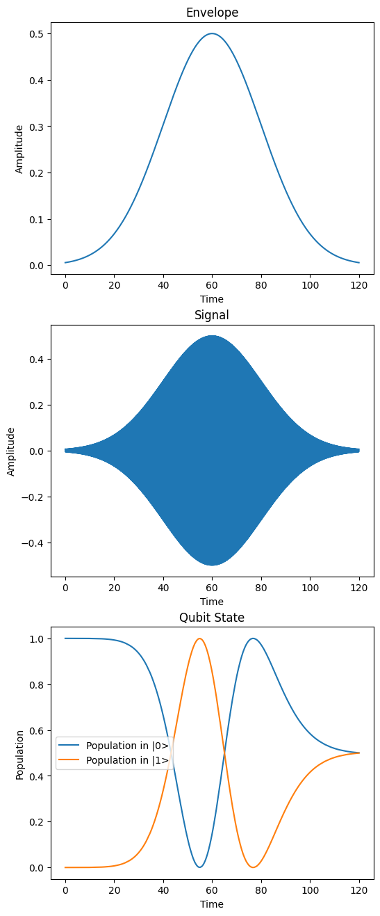
Pulse

This example demonstrates how a transmon qubit is driven by a pulse (modulated signal with a Gaussian envelop) in the lab frame.

import cudaq
from cudaq import spin, boson, ScalarOperator, Schedule, ScipyZvodeIntegrator
import numpy as np
import cupy as cp
import os
import matplotlib.pyplot as plt

# Set the target to our dynamics simulator
cudaq.set_target("dynamics")

# Device parameters
# Strength of the Rabi-rate in GHz.
rabi_rate = 0.1

# Frequency of the qubit transition in GHz.
omega = 5.0 * 2 * np.pi

# Define Gaussian envelope function to approximately implement a `rx(pi/2)` gate.
amplitude = 1. / 2.0  # Pi/2 rotation
sigma = 1.0 / rabi_rate / amplitude
pulse_duration = 6 * sigma


def gaussian(t, duration, amplitude, sigma):
    # Gaussian envelope function
    return amplitude * np.exp(-0.5 * (t - duration / 2)**2 / (sigma)**2)


def signal(t):
    # Modulated signal
    return np.cos(omega * t) * gaussian(t, pulse_duration, amplitude, sigma)


# Qubit Hamiltonian
hamiltonian = omega * spin.z(0) / 2
# Add modulated driving term to the Hamiltonian
hamiltonian += np.pi * rabi_rate * ScalarOperator(signal) * spin.x(0)

# Dimensions of sub-system. We only have a single degree of freedom of dimension 2 (two-level system).
dimensions = {0: 2}

# Initial state of the system (ground state).
psi0 = cudaq.State.from_data(cp.array([1.0, 0.0], dtype=cp.complex128))

# Schedule of time steps.
# Since this is a lab-frame simulation, the time step must be small to accurately capture the modulated signal.
dt = 1 / omega / 20
n_steps = int(np.ceil(pulse_duration / dt)) + 1
steps = np.linspace(0, pulse_duration, n_steps)
schedule = Schedule(steps, ["t"])

# Run the simulation.
# First, we run the simulation without any collapse operators (no decoherence).
evolution_result = cudaq.evolve(hamiltonian,
                                dimensions,
                                schedule,
                                psi0,
                                observables=[boson.number(0)],
                                collapse_operators=[],
                                store_intermediate_results=cudaq.IntermediateResultSave.EXPECTATION_VALUE,
                                integrator=ScipyZvodeIntegrator())

pop1 = [
    exp_vals[0].expectation()
    for exp_vals in evolution_result.expectation_values()
]
pop0 = [1.0 - x for x in pop1]
fig = plt.figure(figsize=(6, 16))
envelop = [gaussian(t, pulse_duration, amplitude, sigma) for t in steps]

plt.subplot(3, 1, 1)
plt.plot(steps, envelop)
plt.ylabel("Amplitude")
plt.xlabel("Time")
plt.title("Envelope")

modulated_signal = [
    np.cos(omega * t) * gaussian(t, pulse_duration, amplitude, sigma)
    for t in steps
]
plt.subplot(3, 1, 2)
plt.plot(steps, modulated_signal)
plt.ylabel("Amplitude")
plt.xlabel("Time")
plt.title("Signal")

plt.subplot(3, 1, 3)
plt.plot(steps, pop0)
plt.plot(steps, pop1)
plt.ylabel("Population")
plt.xlabel("Time")
plt.legend(("Population in |0>", "Population in |1>"))
plt.title("Qubit State")

Text(0.5, 1.0, 'Qubit State')

Qubit Control

This example simulates time evolution of a qubit (transmon) being driven close to resonance in the presence of noise (decoherence) and exhibiting Rabi oscillations.

import cudaq
from cudaq import spin, ScalarOperator, Schedule, ScipyZvodeIntegrator
import numpy as np
import cupy as cp
import os
import matplotlib.pyplot as plt

# Set the target to our dynamics simulator
cudaq.set_target("dynamics")

# Qubit Hamiltonian reference: https://qiskit-community.github.io/qiskit-dynamics/tutorials/Rabi_oscillations.html
# Device parameters
# Qubit resonant frequency
omega_z = 10.0 * 2 * np.pi
# Transverse term
omega_x = 2 * np.pi
# Harmonic driving frequency
# Note: we chose a frequency slightly different from the resonant frequency to demonstrate the off-resonance effect.
omega_drive = 0.99 * omega_z

# Qubit Hamiltonian
hamiltonian = 0.5 * omega_z * spin.z(0)
# Add modulated driving term to the Hamiltonian
hamiltonian += omega_x * ScalarOperator(
    lambda t: np.cos(omega_drive * t)) * spin.x(0)

# Dimensions of sub-system. We only have a single degree of freedom of dimension 2 (two-level system).
dimensions = {0: 2}

# Initial state of the system (ground state).
rho0 = cudaq.State.from_data(
    cp.array([[1.0, 0.0], [0.0, 0.0]], dtype=cp.complex128))

# Schedule of time steps.
t_final = np.pi / omega_x
dt = 2.0 * np.pi / omega_drive / 100
n_steps = int(np.ceil(t_final / dt)) + 1
steps = np.linspace(0, t_final, n_steps)
schedule = Schedule(steps, ["t"])

# Run the simulation.
# First, we run the simulation without any collapse operators (no decoherence).
evolution_result = cudaq.evolve(hamiltonian,
                                dimensions,
                                schedule,
                                rho0,
                                observables=[spin.x(0),
                                             spin.y(0),
                                             spin.z(0)],
                                collapse_operators=[],
                                store_intermediate_results=cudaq.IntermediateResultSave.EXPECTATION_VALUE,
                                integrator=ScipyZvodeIntegrator())

# Now, run the simulation with qubit decoherence
gamma_sm = 4.0
gamma_sz = 1.0
evolution_result_decay = cudaq.evolve(
    hamiltonian,
    dimensions,
    schedule,
    rho0,
    observables=[spin.x(0), spin.y(0), spin.z(0)],
    collapse_operators=[
        np.sqrt(gamma_sm) * spin.plus(0),
        np.sqrt(gamma_sz) * spin.z(0)
    ],
    store_intermediate_results=cudaq.IntermediateResultSave.EXPECTATION_VALUE,
    integrator=ScipyZvodeIntegrator())

get_result = lambda idx, res: [
    exp_vals[idx].expectation() for exp_vals in res.expectation_values()
]
ideal_results = [
    get_result(0, evolution_result),
    get_result(1, evolution_result),
    get_result(2, evolution_result)
]
decoherence_results = [
    get_result(0, evolution_result_decay),
    get_result(1, evolution_result_decay),
    get_result(2, evolution_result_decay)
]

fig = plt.figure(figsize=(18, 6))

plt.subplot(1, 2, 1)
plt.plot(steps, ideal_results[0])
plt.plot(steps, ideal_results[1])
plt.plot(steps, ideal_results[2])
plt.ylabel("Expectation value")
plt.xlabel("Time")
plt.legend(("Sigma-X", "Sigma-Y", "Sigma-Z"))
plt.title("No decoherence")

plt.subplot(1, 2, 2)
plt.plot(steps, decoherence_results[0])
plt.plot(steps, decoherence_results[1])
plt.plot(steps, decoherence_results[2])
plt.ylabel("Expectation value")
plt.xlabel("Time")
plt.legend(("Sigma-X", "Sigma-Y", "Sigma-Z"))
plt.title("With decoherence")

Text(0.5, 1.0, 'With decoherence')

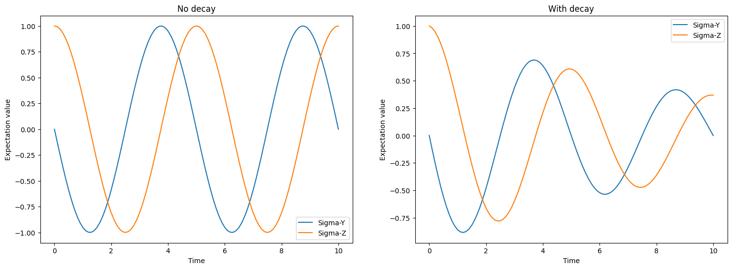
Qubit Dynamics

import cudaq
from cudaq import spin, Schedule, RungeKuttaIntegrator
import numpy as np
import cupy as cp
import os
import matplotlib.pyplot as plt

# Set the target to our dynamics simulator
cudaq.set_target("dynamics")

# Qubit Hamiltonian
hamiltonian = 2 * np.pi * 0.1 * spin.x(0)

# Dimensions of sub-system. We only have a single degree of freedom of dimension 2 (two-level system).
dimensions = {0: 2}

# Initial state of the system (ground state).
rho0 = cudaq.State.from_data(
    cp.array([[1.0, 0.0], [0.0, 0.0]], dtype=cp.complex128))

# Schedule of time steps.
steps = np.linspace(0, 10, 101)
schedule = Schedule(steps, ["time"])

# Run the simulation.
# First, we run the simulation without any collapse operators (ideal).
evolution_result = cudaq.evolve(hamiltonian,
                                dimensions,
                                schedule,
                                rho0,
                                observables=[spin.y(0), spin.z(0)],
                                collapse_operators=[],
                                store_intermediate_results=cudaq.IntermediateResultSave.EXPECTATION_VALUE,
                                integrator=RungeKuttaIntegrator())

# Now, run the simulation with qubit decaying due to the presence of a collapse operator.
evolution_result_decay = cudaq.evolve(
    hamiltonian,
    dimensions,
    schedule,
    rho0,
    observables=[spin.y(0), spin.z(0)],
    collapse_operators=[np.sqrt(0.05) * spin.x(0)],
    store_intermediate_results=cudaq.IntermediateResultSave.EXPECTATION_VALUE,
    integrator=RungeKuttaIntegrator())

get_result = lambda idx, res: [
    exp_vals[idx].expectation() for exp_vals in res.expectation_values()
]
ideal_results = [
    get_result(0, evolution_result),
    get_result(1, evolution_result)
]
decay_results = [
    get_result(0, evolution_result_decay),
    get_result(1, evolution_result_decay)
]

fig = plt.figure(figsize=(18, 6))

plt.subplot(1, 2, 1)
plt.plot(steps, ideal_results[0])
plt.plot(steps, ideal_results[1])
plt.ylabel("Expectation value")
plt.xlabel("Time")
plt.legend(("Sigma-Y", "Sigma-Z"))
plt.title("No decay")

plt.subplot(1, 2, 2)
plt.plot(steps, decay_results[0])
plt.plot(steps, decay_results[1])
plt.ylabel("Expectation value")
plt.xlabel("Time")
plt.legend(("Sigma-Y", "Sigma-Z"))
plt.title("With decay")

Text(0.5, 1.0, 'With decay')

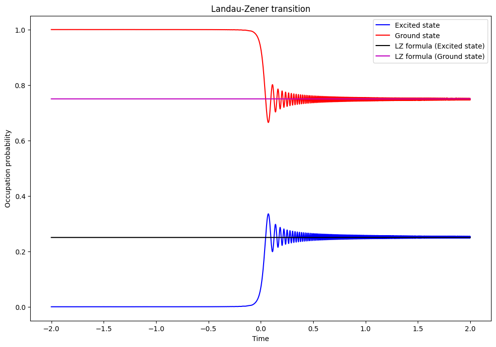
Landau-Zenner

This example simulates the so-called Landau–Zener transition: given a time-dependent Hamiltonian such that the energy separationof the two states is a linear function of time, an analytical formula exists to calculate the probability of finding the system in the excited state after the transition.

import cudaq
from cudaq import spin, boson, ScalarOperator, Schedule, ScipyZvodeIntegrator
import numpy as np
import cupy as cp
import os
import matplotlib.pyplot as plt

# References:
# - https://en.wikipedia.org/wiki/Landau%E2%80%93Zener_formula
# - `The Landau-Zener formula made simple`, `Eric P Glasbrenner and Wolfgang P Schleich 2023 J. Phys. B: At. Mol. Opt. Phys. 56 104001`
# - QuTiP notebook: https://github.com/qutip/qutip-notebooks/blob/master/examples/landau-zener.ipynb

# Set the target to our dynamics simulator
cudaq.set_target("dynamics")

# Define some shorthand operators
sx = spin.x(0)
sz = spin.z(0)
sm = boson.annihilate(0)
sm_dag = boson.create(0)

# Dimensions of sub-system. We only have a single degree of freedom of dimension 2 (two-level system).
dimensions = {0: 2}

# Landau–Zener Hamiltonian:
# `[[-alpha*t, g], [g, alpha*t]] = g * pauli_x - alpha * t * pauli_z`
g = 2 * np.pi
# Analytical equation:
# `P(0) = exp(-pi * g ^ 2/ alpha)`
# The target ground state probability that we want to achieve
target_p0 = 0.75
# Compute `alpha` parameter:
alpha = (-np.pi * g**2) / np.log(target_p0)

# Hamiltonian
hamiltonian = g * sx - alpha * ScalarOperator(lambda t: t) * sz

# Initial state of the system (ground state)
psi0 = cudaq.State.from_data(cp.array([1.0, 0.0], dtype=cp.complex128))

# Schedule of time steps (simulating a long time range)
steps = np.linspace(-2.0, 2.0, 5000)
schedule = Schedule(steps, ["t"])

# Run the simulation.
evolution_result = cudaq.evolve(hamiltonian,
                                dimensions,
                                schedule,
                                psi0,
                                observables=[boson.number(0)],
                                collapse_operators=[],
                                store_intermediate_results=cudaq.IntermediateResultSave.EXPECTATION_VALUE,
                                integrator=ScipyZvodeIntegrator())

prob1 = [
    exp_vals[0].expectation()
    for exp_vals in evolution_result.expectation_values()
]

prob0 = [1 - val for val in prob1]
fig, ax = plt.subplots(figsize=(12, 8))
ax.plot(steps, prob1, 'b', steps, prob0, 'r')
ax.plot(steps, (1.0 - target_p0) * np.ones(np.shape(steps)), 'k')
ax.plot(steps, target_p0 * np.ones(np.shape(steps)), 'm')
ax.set_xlabel("Time")
ax.set_ylabel("Occupation probability")
ax.set_title("Landau-Zener transition")
ax.legend(("Excited state", "Ground state", "LZ formula (Excited state)",
           "LZ formula (Ground state)"),
          loc=0)

<matplotlib.legend.Legend at 0x7fa9f4718af0>