Quantum-Selected Configuration Interaction (QSCI)

Quantum-Selected Configuration Interaction (QSCI) [1] is a quantum-classical hybrid algorithm designed for electronic structure calculations, particularly to compoute ground state and excited state energies of molecular systems. This method is one of the quantum subspace diagonalization (QSD). It is well-suited for NISQ-era quantum devices, focusing on using quantum resources efficiently while maintaining high accuracy.

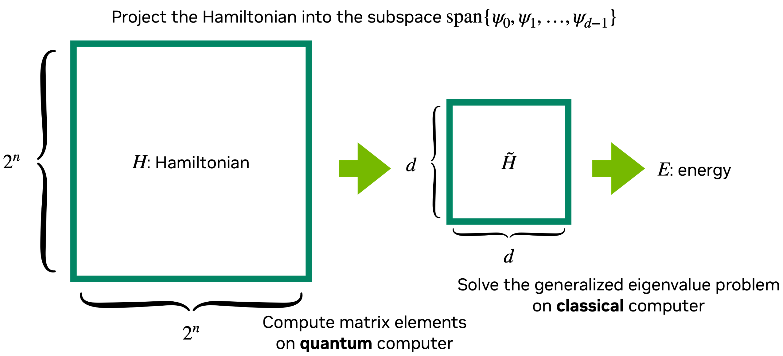
QSCI selects this vector space from a sampled computational basis.

0. Problem definition

Let’s define Hamiltonian of \(\mathrm{H_4}\).

!pip install --quiet --break-system-packages openfermionpyscf==0.5

import openfermion
import openfermionpyscf
from openfermion.transforms import jordan_wigner, get_fermion_operator
import cudaq

# Number of hydrogen atoms.
hydrogen_count = 4

# Distance between the atoms in Angstroms.
bond_distance = 0.7474

# Define a linear chain of Hydrogen atoms
geometry = [("H", (0, 0, i * bond_distance)) for i in range(hydrogen_count)]

basis = "sto3g"
multiplicity = 1
charge = 0

molecule = openfermionpyscf.run_pyscf(
    openfermion.MolecularData(geometry, basis, multiplicity, charge), run_fci=True
)
molecular_hamiltonian = molecule.get_molecular_hamiltonian()
fermion_hamiltonian = get_fermion_operator(molecular_hamiltonian)
qubit_hamiltonian = jordan_wigner(fermion_hamiltonian)
qubit_hamiltonian.compress()

hamiltonian = cudaq.SpinOperator(qubit_hamiltonian)

num_qubits = hamiltonian.qubit_count
electron_count = molecule.n_electrons

1. Prepare an Approximate Quantum State

Start with a variational ansatz (e.g., from VQE) to approximate the ground state wavefunction on a quantum computer.

import numpy as np


@cudaq.kernel
def kernel(thetas: list[float]):

    qubits = cudaq.qvector(num_qubits)

    # Hartree-Fock
    for i in range(electron_count):
        x(qubits[i])
    # UCCSD
    cudaq.kernels.uccsd(qubits, thetas, electron_count, num_qubits)


parameter_count = cudaq.kernels.uccsd_num_parameters(electron_count, num_qubits)


from scipy.optimize import minimize


# Define a function to minimize
def cost(thetas: list[float]):
    exp_val = cudaq.observe(kernel, hamiltonian, thetas).expectation()
    return exp_val


exp_vals = []


def callback(xk):
    exp_vals.append(cost(xk))


# Initial variational parameters.
np.random.seed(15)
x0 = np.random.normal(0, np.pi, parameter_count)

# Use the scipy optimizer to minimize the function of interest
vqe_result = minimize(cost, x0)

2 Quantum Sampling to Select Configuration

Measure this quantum state multiple times to obtain bitstrings, which correspond to Slater determinants (electronic configurations).

sample_result = cudaq.sample(kernel, vqe_result.x)
print(sample_result)

{ 00001111:2 00011011:12 00011110:18 00100111:27 00101101:25 00110011:2 00110110:22 00111001:193 01011010:13 01101100:23 01110010:2 10000111:34 10001101:115 10010011:18 10010110:5 10011100:11 10100101:40 10110001:4 11000011:170 11001001:16 11001100:8 11010010:46 11011000:137 11100001:7 11100100:28 11110000:22 }

3. Classical Diagonalization on the Selected Subspace

Construct a truncated Hamiltonian matrix using only the selected determinants. Diagonalize this matrix classically to obtain improved energy estimates.

def pauli_element(
    operator: cudaq.SpinOperator, b1: str | np.ndarray, b2: str | np.ndarray
) -> complex:
    """
    Compute an inner product <b1|operator|b2>.
    """

    if isinstance(b1, str):
        b1 = np.array([i == "1" for i in b1], dtype=bool)
    if isinstance(b2, str):
        b2 = np.array([i == "1" for i in b2], dtype=bool)

    num_qubits = hamiltonian.qubit_count
    num_terms = hamiltonian.term_count

    bsv = np.zeros((num_terms, 2 * num_qubits), dtype=bool)
    coeffs = np.zeros(num_terms, dtype=np.complex128)
    for i, term in enumerate(operator):
        coeffs[i] = term.evaluate_coefficient()
        bsf = term.get_binary_symplectic_form()
        n = len(bsf) // 2
        for j, e in enumerate(bsf):
            if j < n:
                bsv[i, j] = e
            else:
                bsv[i, j - n + num_qubits] = e
    x = bsv[:, :num_qubits]
    z = bsv[:, num_qubits:]

    # b1 ⊕ b2 must match x for nonzero contribution
    delta = np.bitwise_xor(b1, b2)
    match = np.all(x == delta, axis=1)

    if not np.any(match):
        return 0.0

    matched_x = x[match]
    matched_z = z[match]
    matched_coeffs = coeffs[match]

    # i^{x·z}
    x_dot_z = np.sum(np.bitwise_and(matched_x, matched_z), axis=1) % 4
    i_phases = np.array([1, 1j, -1, -1j], dtype=np.complex128)[x_dot_z]

    # (-1)^{b1·z}
    b1_dot_z_parity = np.sum(np.bitwise_and(b1, matched_z), axis=1) % 2
    sign_phases = np.where(b1_dot_z_parity == 0, 1, -1)

    result_terms = matched_coeffs * i_phases * sign_phases
    return np.sum(result_terms)

import scipy

bitstrs = list(k for k, _ in sample_result.items())
subspace_dimension = len(bitstrs)

values = []
row_ids = []
column_ids = []

for i in range(subspace_dimension):
    for j in range(i, subspace_dimension):
        elem = pauli_element(hamiltonian, bitstrs[i], bitstrs[j])
        if abs(elem) > 1e-6:
            values.append(elem)
            row_ids.append(i)
            column_ids.append(j)
            if i != j:
                values.append(elem.conjugate())
                row_ids.append(j)
                column_ids.append(i)

values = np.real_if_close(values)

truncated_hamiltonian = scipy.sparse.coo_array(
    (values, (row_ids, column_ids)), shape=(subspace_dimension, subspace_dimension)
)
eigvals, _ = scipy.sparse.linalg.eigsh(truncated_hamiltonian, 1, which="SA")

5. Compuare results

## QSCI
eigvals[0]

-2.1318697852134716

## FCI Energy
molecule.fci_energy

-2.143554580446029

Reference

[1] “Quantum-selected configuration interaction: classical diagonalization of hamiltonians in subspaces selected by quantum computers” K. Kanno, M. Kohda, R. Imai, S. Koh, K. Mitarai, W. Mizukami, and Y. O. Nakagawa (2023) arXiv: 2302.11320